Cumulative trophic curves elucidate tropical coral reef ecosystems

1 Introduction

The search and identification of repeatable and predictable patterns remains an important driver in ecological sciences (Peters, 1991). Specifically, the question remains whether there are common patterns of ecosystems that arise from consistent, underlying, fundamental ecosystem processes (Jorgensen, 2009). A few have been posited (Harfoot et al., 2014). Yet whether such emergent patterns are germane for marine ecosystems remains unclear due to the distinctiveness of the marine environment (Steele, 1985; de Young et al., 2004). Finding such patterns that are robust and widespread is not trivial. Being able to elucidate the determinants of such patterns, and how they respond under differing environmental conditions and pressures, is also not trivial.

One approach, which emphasizes such emergent patterns, hypothesizes that the cumulative trophic theory exhibits robust and widespread patterns in all marine ecosystems (see Pranovi and Link, 2009; Pranovi et al., 2012; Pranovi et al., 2014; Link et al., 2015; Libralato et al., 2019; Link et al., 2020; Pranovi et al., 2020). These emergent features are based on observations and supporting theory that biomass accumulation is (log-) normally distributed and represents transfer (even if inefficiently) of biomass and hence production up a food web to successive trophic levels (Link et al., 2015). Fundamental trophodynamic features— overall system limits based on primary production, turn-over of populations, average growth efficiency— are the overall system limits that influence the production curve (c.f., Link et al., 2015). Furthermore, biomass accumulation across trophic level is not inevitably pyramidal in marine systems but is more often rhomboidal due to high standing biomass at TL 2 (i.e., benthos and plankton; Link et al., 2015); thus, the cumulative biomass curve across trophic levels (cumB-TL) is a sigmoidal curve (i.e., a curve with a clear inflection point indicative of this rhomboidal pattern (Figure 1)). These represent emergent features of ecosystems that have high potential utility, both for better understanding reef status and even informing management options thereon. In particular, the cumulative biomass-trophic level curves result in S-curves which are consistent and widespread, repeated in every marine ecosystem examined from over 200 different ecosystems for over 70 years of observations (Link et al., 2015; Libralato et al., 2019). These cumulative curves also show clear, repeatable, and predictable patterns when a marine ecosystem is undergoing perturbation, to the point that thresholds have been proposed based on these curve properties (Link et al., 2015; Libralato et al., 2019; Pranovi et al., 2020). In the cumulative trophic context, marine ecosystems essentially follow the pattern that as an ecosystem experiences perturbation, the S-curve shrinks and moves closer to the origin, which is captured in the various curve parameters of cumulative biomass and production curves. In many respects these emergent features integrate over an entire food web (Link et al., 2015).

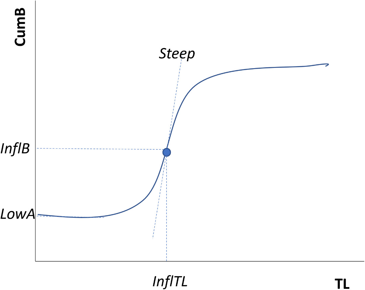
Figure 1 Example of the Cumulative Biomass curve and the 4 parameters used for describing it; Steep, steepness (the slope of the tangent passing through the inflection point); InflTL, TL of the inflection point (the point of change in the slope curvature of the S curve, projected onto the x‐axis); InflB, % biomass of the inflection point (the point of change in the slope curvature of the S‐curve, projected onto the y‐axis) and LowA, the lower asymptote (the point of interception of the curve on the y-axis). Adapted from Link et al. (2015).

The cumulative trophic theory has been tested for hundreds of different (and different types of) marine ecosystem (Link et al., 2015; Libralato et al., 2019), the patterns appear to be robust, and the S-curves and associated curve parameters respond to pressures in a predictable manner. The S-curves have mostly been developed and tested for larger marine ecosystems, and most have been examined for continental shelf, upwelling, small sea, open ocean, and estuarine ecosystems. The original work did have a few coral reef ecosystems which exhibited similar but less consistent cumulative theory patterns. Yet the robustness, predictability, repeatability, and determinants of S-curves have not been fully tested for coral reef ecosystems.

Implied in the cumulative trophic approach is that it allows one to investigate the structural function of any ecosystem; namely by looking at the community composition with a focus on energy flows as mediated by the system transfer efficiency. We acknowledge that all ecosystems are complex and have unique features to them, and thus there are many potential determinants and characteristics of ecosystem structure and function. But if there are ones that are globally repeatable and widely observed, which we hypothesize the cumulative S-curve to be (Link et al., 2015), that is not trivial.

Coral reef ecosystems are unique among marine ecosystems. Not only are they inherently intriguing with high aesthetic attraction, they represent global hotspots of biodiversity (Reaka-Kudla, 1997; Hughes et al., 2002), provide critical ecosystem (Moberg and Folke, 1999; Barbier et al., 2011) and cultural services for many island communities (see Moberg and Folke, 1999; Whittingham et al., 2003; Cinner, 2014), have a unique balance of endogenous and exogenous production, and support many facets of local, island economies (Whittingham et al., 2003; Burke et al., 2011). Coral reef ecosystems are also facing a plethora of pressures, ranging from bleaching (Hoegh-Guldberg, 1999; Hughes et al., 2003; Baker et al., 2008; Hoegh-Guldberg et al., 2017) to acidification (Langdon and Atkinson, 2005; Pandolfi et al., 2011) to broader warming impacts (Baker et al., 2008; Heron et al., 2016; Hughes et al., 2018) to siltation (due to land-use practices or sedimentation; Rogers, 1990; Dubinsky and Stambler, 1996; Fabricius, 2005; Erftemeijer et al., 2012) to over-exploitation of their living marine resources (Jackson et al., 2001; Newton et al., 2007; Burke et al., 2011) to pollution (Dubinsky and Stambler, 1996; Burke et al., 2011). In general, marine ecosystems, especially coral reefs, provide a wide range of highly visible, desirable, and valuable goods and services, but face significant pressures. A full range of pressures can alter the structure, functioning and resilience of marine ecosystems, and often act in concert to produce cumulative effects (Jackson et al., 2001); hence cumulative evaluations can be useful. Additionally, calls to protect the critical ecosystem functions that coral reef ecosystems deliver (Bellwood et al., 2019) have come alongside advances in monitoring the functions of these systems (e.g., Mouillot et al., 2014, Richardson et al., 2018) which warrants further synthesis of these complex systems. The cumulative trophic approach could provide additional insights and means to elucidate the dynamics of coral reefs.

Here, we aim to test cumulative trophic theory on coral reef ecosystems. We do so by calculating cumulative trophic curves from a wide range of U.S. Pacific Island reef ecosystems, spanning a gradient of human impact and environmental features, including some of the most remote, unfished coral reef ecosystems in the world. We want to explore differences in these cumulative curve properties as they vary across a range of environmental and human conditions. We also want to examine if there are any archipelago-related features common to coral reef ecosystems. We also wanted to explore the determinants of cumulative curve properties relative to various measures of coral reef features. We generally hypothesize that consistent with cumulative trophic theory, those islands experiencing more pressure (as indicated by a variety of measures) will exhibit less pronounced S-curves (and associated parameters) than those that are not. Being able to examine this approach across a suite of over 40 island coral reef ecosystems, using similarly collected data but across a wide range of environmental and perturbation conditions, is expected to have high utility.

2 Materials and methods

2.1 Study area

The study area comprises coral reefs around US- and US-affiliated islands and atolls in the Central and Western Pacific (the Hawaiian and Mariana Archipelagos, the Pacific Remote Island Areas, and American Samoa (Figure 2)), ranging from heavily populated (e.g., Oahu, Maui, Guam, and Tutuila) to extremely remote and uninhabited reef areas several hundred or thousand kilometers from the nearest human population centers. There were 42 island reef ecosystems (listed in Table 1; see also Figure 2) sampled and analyzed in this study.

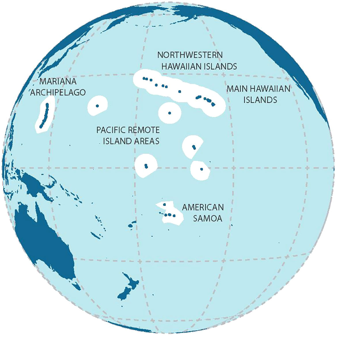
Figure 2 Study areas of major island archipelagoes; used with permission from McCoy et al. (2019); for the list of the islands see Table 1.

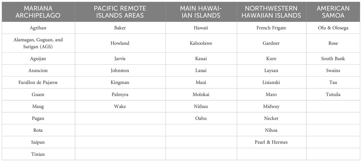
Table 1 List of the islands for each of the archipelagoes.

2.2 Fish survey data and sampling sources

We used the most recent data collected from fish surveys conducted as a component of the National Coral Reef Monitoring Program (NCRMP) across the U.S. Pacific Islands (see Heenan et al., 2018 for detailed methods; see also Brainard et al., 2012; Brainard et al., 2019): Guam and the Commonwealth of Northern Mariana Islands (Mariana, 2017), American Samoa (2018), the Pacific Remote Islands Areas (PRIA, 2018), and the Northwestern (2017) and Main (2019) Hawaiian Islands. Briefly, the NCRMP employs a stratified-random survey design across a domain of hard-bottom habitat in depths of less than 30 m. All islands (and atolls) within regions were stratified by reef zone (backreef, forereef, lagoon, protected slope; mostly forereef) and depth zone (shallow [>0-6 m], mid [>6-18 m], deep [>18-30 m]). The number of random sites per stratum were selected according to the proportional area of each stratum and the variance of target fish groups (e.g., piscivores, herbivores, total fish biomass, etc.) from prior surveys. At each random site, a pair of divers conducted Stationary Point Count (SPC) surveys by counting and sizing (visually estimated total length, to the nearest cm) observed fish within two adjacent 15-m diameter cylindrical plots. Prior to surveys, divers undergo extensive training that includes sizing calibrations with wooden fish cutouts, and diver-to-diver comparisons of fish sizing, species richness, and abundance estimates are conducted throughout the data collection period. These steps (among other QA/QC practices) are used to minimize diver bias across the dataset.

The body weight of each observed fish was estimated using length-to-weight conversion parameters from FishBase (Kulbicki et al., 2005; Froese and Pauly, 2023). Site-level biomass per species was calculated by averaging between paired SPC surveys. To aggregate estimates up to the island level, values were averaged across sites within each stratum, then weighted according to the proportional size of each stratum relative to the total area surveyed of the corresponding island, and then summed across strata within each island.

Given the aims of the present work we decided to maintain all sharks and jacks in the biomass estimates, even if the different responses of those highly mobile, roving piscivores to the presence of divers could be a potential source of bias among study locations (with a possible density overestimation), mainly in remote areas (sensu Heenan et al., 2020; I. Williams, pers. comm.). However, since the presence of these two groups strongly characterizes just those remote systems with high abundances of large predators, we decided to conduct the analyses both with and without these groups, but emphasize and present the former here (including the latter in Supplementary Materials). We also acknowledge that a significant portion of the food web biomass in coral reef ecosystems is sequestered in the benthos (i.e., corals, cryptic-benthic fishes, other invertebrates) but we do not fully treat benthic biomass here. We do consider the proportion of hard bottom as an environmental covariate that in some ways proxies coral coverage, albeit imperfectly. This limited benthic treatment could perhaps alter the shape and parameters of the S-curves. But our experience from other ecosystems (Libralato et al., 2019; Pranovi et al., 2020) does not negate the still largely systematic, and we argue insightful, view that cumulative biomass curves based on non-benthos and mostly fish biomass can provide.

2.3 Island level human and environmental characterization

To determine the generalizable nature of the cumulative biomass (cumB) curves we investigated how the curve indicator parameter estimates varied in relation to gradients in oceanographic condition and human impact. The cumB curves were calculated at the island ecosystem scale (one curve per island), and paired with island level estimates of human population density and biophysical drivers (Table 2) that we expected a priori to influence the standing biomass of fishes observed at these locations. While is it clear that sub-island variation significantly influences fish biomass observed within a region (Gorospe et al., 2018), here we use the large, pan-Pacific nature of this monitoring dataset and the spatial gradients it spans to assess the utility of the cumB approach as an indicator at the ecosystem scale. Other studies (Williams et al., 2015; Heenan et al., 2020) have demonstrated that the larger oceanographic context surrounding these islands is not trivial, and that inter-island contrast is primarily what we wanted to explore versus intra-island variance. Thus, here we present the islands as associated with the mean values of some relevant environmental conditions to characterize them relative to their position along oceanographic gradients and levels of human impacts.

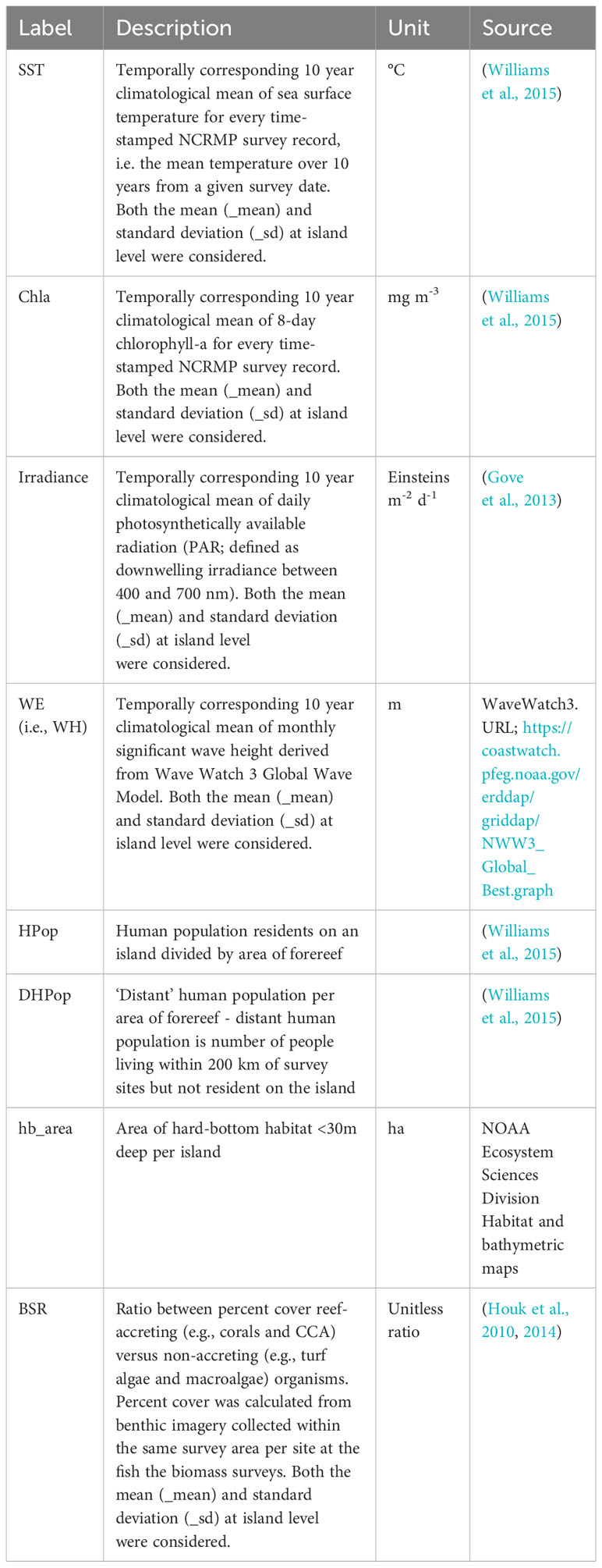
Table 2 Environmental variables considered for the characterization of the islands.

Two different scales of human impact were investigated, local human population density and distant human population density (Table 2). These metrics are coarse proxies for overall human impacts, including fishing. Local human population density at these islands correlates well with distance to provincial capital (Heenan et al., 2016), a metric which in the absence of direct measures of fishing effort on coral reef fishes, is used as a proxy for fisheries impacts (Brewer et al., 2013; Cinner et al., 2013; Maire et al., 2016). We assume it also characterizes other indirect effects of humans on these ecosystems, such as land-based sources of pollution. Initially, human population density was treated as a continuous variable but for subsequent inferential analysis, we binned these data. Rather than having a binary populated or unpopulated division, which would group the most heavily populated places with the remote locations with very limited human presence, we binned islands into those which were lightly populated (none-low; 0-100 people per hectare of reef) and populated (mid-high; >100 people per hectare of reef).

The biophysical oceanographic drivers investigated here were based on numerous studies that have used the Pacific NCRMP dataset, and found to have an important influence on coral reef fish biomass (Williams et al., 2015; Cinner et al., 2016; Heenan et al., 2016; Robinson et al., 2017; Heenan et al., 2020). These drivers represent estimates of the prevailing oceanographic conditions derived from remotely-sensed data. Temporally corresponding climatologies over 10 years for every time-stamped and georeferenced NCRMP survey record were calculated for significant wave height, sea-surface temperature (SST), the photic and hence production conditions (photosynthetically active radiation; PAR) and oceanic productivity (chlorophyll-a), and a proxy for coral coverage (hard-bottom habitat, as compared to other, softer substrates like algae or sand). The resolution of the gridded remotely-sense data was coarser than the expected accuracy of most survey site locations (<5 km), so horizontal positions were matched to the nearest available gridded data within 0.1°. Monthly significant wave height data (1979-2020) was derived from the WaveWatch III Global Wave Model at a resolution of 0.4°. Daily SST data (1985-2020) was gathered from the NOAA Coral Reef Watch program (v1.0) with a resolution of 0.05°. 8-day surface chlorophyll-a concentrations (1997-2020) were derived from the European Space Agency Ocean Color Climate Change Initiative (ESA OC CCI; v5.0) at a resolution of 0.042°. Daily PAR (2002-2020) was obtained from Moderate Resolution Imaging Spectroradiometer Aqua (Aqua MODIS: v.2018.0) with a resolution of 0.042°. Remotely-sensed ocean color data (PAR and chlorophyll-a) were masked at original resolution (i.e., pixel-level) as a quality control measure (Winston et al., 2022). First, the gridded ocean color data were overlaid over high resolution bathymetry data (15 arc seconds; Becker et al., 2009). Second, any ocean color pixels with an area greater than 5% characterized in depths of 30 m or shallower were masked. Subsequent climatological analyses for NCRMP survey sites were performed using the ocean color values extracted from the nearest pixel. We also acknowledge that the irradiance and chlorophyll might not fully capture all the production dynamics on reefs, but do largely capture the broader oceanographic context that each island resides within. We use summary climatologies here, designed to compress the influence of anomalous conditions experienced across the time series from which they were calculated, in order to characterize the broad oceanographic contexts across the large sample frame of 42 degrees (°) of latitude (14° S to 28° N), and 62° of longitude (178° W to 145° E).

In addition to the human and oceanographic features, we characterize each reef with the benthic substrate ratio (BSR) as a measure of reef condition (e.g., Houk et al., 2010; Houk et al., 2014). This ratio is the percent cover of reef-accreting (e.g., corals and crustose coralline algae (CCA)) divided by the percent cover of non-accreting (e.g., turf, encrusting and macroalgae) benthic organisms. We also consider the standard deviation for the BSR values to provide a sense of island-level variability. Benthic composition (percent cover of broad functional groups) was calculated from photoquadrats imaged at every 1-m mark along a 30-m transect over which each pair of fish SPC cylinders were centered, resulting in a total of 30 photoquadrat images collected per survey site. These images were annotated using the web-based software, CoralNet (Beijbom et al., 2015; Williams et al., 2019). Site-level estimates of percent cover of the following functional groups were calculated: macroalgae, turf algae, coral, CCA, sand. The cover of calcifying versus non-calcifying groups were summed and used to calculate BSR values per site. These site level estimates were then pooled to island-scale mean and standard deviations using the same weighting procedure described above for the fish data.

2.4 Cumulative curve parameters

To characterize the properties of each cumulative curve, or the S-curve of cumulative biomass relative to trophic level (Figure 1), four parameters were estimated for a logistic model of the cumulative biomass. These were the steepness of the curve (Steep) which mathematically is the slope of the tangent passing through the inflection point. The steepness measure gives a sense of how compressed or stretched out, corresponding to perturbed or recovering/functional respectively, an S-curve is as has been noted previously (Figure 1; Link et al., 2015; Libralato et al., 2019). The trophic level at the inflection point (InflTL) is where the point of the second derivative changes sign in the slope curvature as projected onto the x‐axis. This is generally interpreted as the lower an InflTL value, the more concerning the curve might be, with thresholds at mid-TLs usually apparent (Libralato et al., 2019). The percentage of biomass at the inflection point (InflB) is the point of change in the slope curvature of the S‐curve projected onto the y‐axis. Usually any value below ~33% indicates a highly perturbed ecosystem (Libralato et al., 2019). The lower asymptote (LowA) is a new parameter we estimate here and is the point of interception of the curve on the y-axis. It essentially indicates the basal biomass (and implied production) of an ecosystem.

2.5 Data analyses

Species estimates of trophic level were obtained from FishBase (Froese and Pauly, 2010), and fish biomass per island were summed to discrete trophic level (TL) intervals (interval width: 0.1 TL) to build the cumulative curve of biomass versus TL (Link et al., 2015). Data were then fit independently for each island, with a four‐parameter logistic nonlinear regression model (Ricketts and Head, 1999) using the ‘drc’ package (Ritz, et al., 2015) within the R statistical environment (v. 4.0.5; R Core Team, 2021) according to the methods used by Pranovi et al. (2014). Again, the S‐curve parameters —steepness (the slope of the tangent passing through the inflection point; Steep), TL of the inflection point (the point of change in the slope curvature of the S curve, projected onto the x‐axis; InflTL), % biomass of the inflection point (the point of change in the slope curvature of the S‐curve, projected onto the y‐axis; InflB) and the lower asymptote (the point of interception of the curve on the y-axis; LowA)—were estimated through a best fit process, fixing the upper asymptote to 1 (to normalize across islands). Again, perturbations to these ecosystems result in changes in the S-curve over time that become less steep and move toward lower TLs. Conversely, ecosystem recovery results in increased steepness and movement toward upper TLs of these curves (Link et al., 2015).

As previous studies have shown that biomass distribution across trophic levels can be related to environmental features, human density, and reef status (Williams et al., 2015; Heenan et al., 2016; Gorospe et al., 2018; Heenan et al., 2020), we also computed simple indicators to summarize the main characteristics of the fish assemblage and used them to compare with the S-curve parameters. These assemblage indicators are: the total number of fish species (S), the total biomass (Btot), the mean trophic level (meanTL), the biomass of fish with trophic level between 2 and 3 (B_2_3), and the proportion of the total biomass of fish with trophic level between 2 and 3 (Prop.2_3), the biomass of fish with trophic level between 3 and 4 (B_3_4) and the proportion of the total biomass of fish with trophic level between 3 and 4 (Prop.3_4), the biomass of fish with trophic level between 4 and 5 (B_4_5), and the proportion of the total biomass of fish with trophic level between 4 and 5 (Prop.4_5).

To understand the influence that migratory, upper trophic level species may have on the curve parameters, the analysis was run twice, once with all species included and again without sharks and jacks (sensu Williams et al., 2015). The potential impacts of particular species were further investigated using a jackknife-based resampling procedure to assess the influence of a given species in the uncertainty of the curve estimates. For each island, the curve fitting procedure was replicated by systematically leaving out one species. This provided an assessment of both the uncertainty of fitting and contribution of each species to the uncertainty of the S-curve parameters.

The characteristics of the islands were explored following a multivariate analysis approach in two steps: a) first an unconstrained ordination (Principal Component Analysis; PCA) on standardized variables (mean centered and scaled with standard deviation) was used to understand the placement of the islands within the gradients of environmental features and human pressures; b) second, a constrained ordination (redundancy analysis; RDA) using the parameters of the S-curves and the assemblage indicators as response variables, in order to understand the role of the aforementioned environmental and human pressure gradients on the characteristics of the fish assemblage and hence on the shape of the curves. Essentially, we were seeking to ascertain any gradients in environmental and human factors which might drive the features of cumulative curve parameters. Multivariate analyses were performed using the vegan package (Oksanen et al., 2020) for R. The curve parameters, for all the 42 islands, were explored in relation to human pressure with a particular attention to the role of human population, that has been classified considering two levels: no to low level of human population (0-100 people per hectare) and mid to high level (> 100 people) per hectare. We acknowledge that populations >100 can span quite a range, but our aim here was to essentially delineate populated and non-populated islands. The explainable variance in these analyses was reported, with the aim of elucidating some of the major distinctions in cumulative biomass curves for across these trophic coral reefs.

3 Results

Generally, the curves show the expected S-shape pattern, representing the distribution of biomass accumulation across TL (Figure 3). These S-curves vary across islands, as would be expected. Namely, there is a degree of variability in the shape of the curves (Figure 3) and hence in its parameters (Supplementary Figure S1); part of such variability can be ascribed to differences among regions, but other factors may also influence this variability. The logistic curves seem to fit robustly, except for just a few islands exhibiting higher uncertainty. These are mostly associated with curves showing high steepness, namely French Frigate, Gardner, Kure, Lisianski, Midway, Pearl & Hermes, and South Bank, not related to a particular archipelago region (Figure 2). Also noteworthy is that some S-curves are more pronounced (Figure 3; i.e., higher steepness (slope) and higher inflection point parameters), indicative of less perturbed conditions. All of these occur at less populated islands.

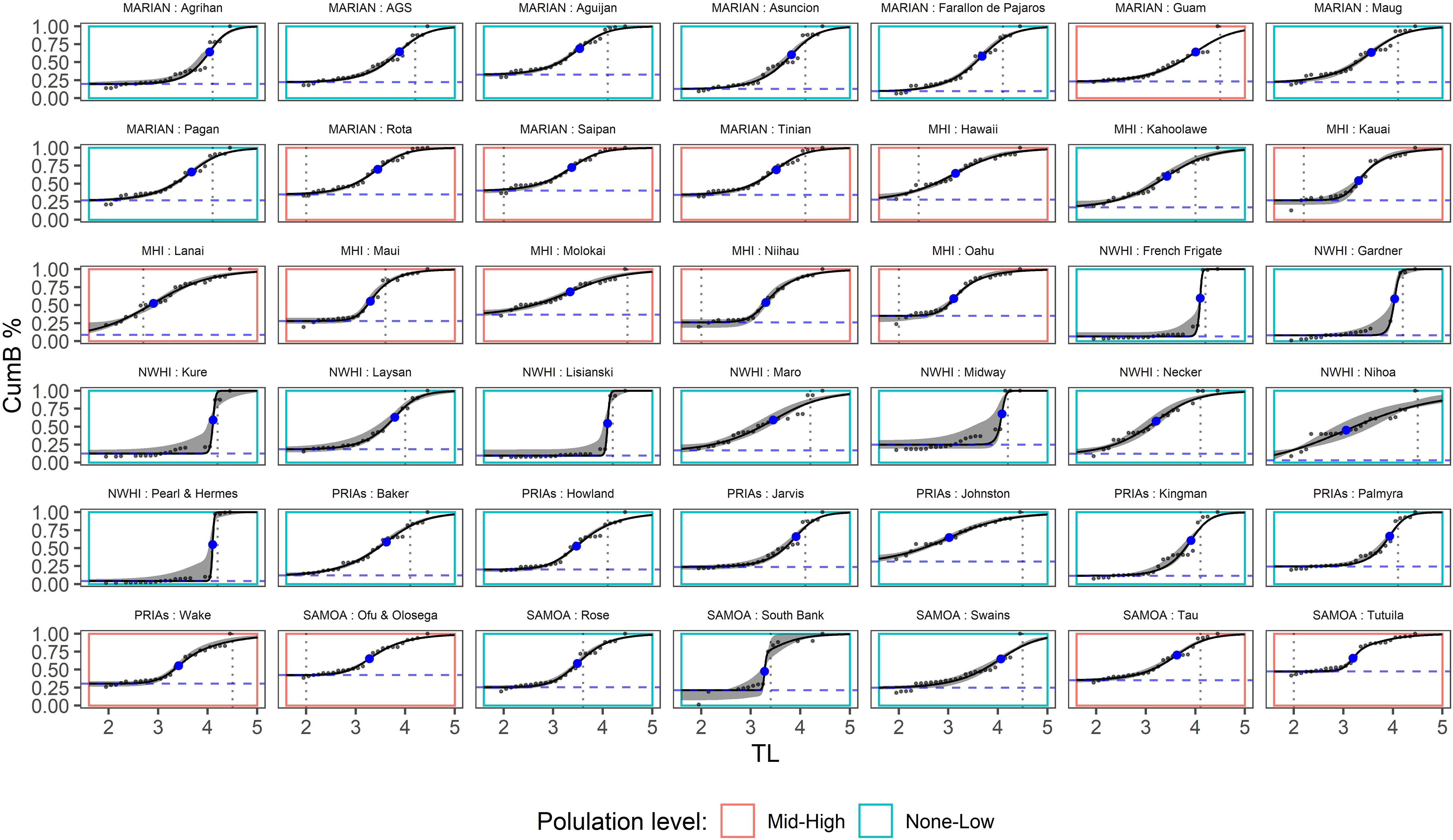
Figure 3 Cumulative biomass across trophic level (TL; black lines) and 99% confidence interval calculated with the Jackknife procedure (see Analyses section in the main text). Vertical dotted lines represent the TL of the fish species most contributing to the uncertainty; the blue points represent the inflection points; horizontal dashed blue line represent the lower intercept; the colored rectangle represents the population level, as defined in the text; Marian, Mariana Archipelago; MHI, Main Hawaiian islands; NWHI, Northwestern Hawaiian Islands; PRIAs, Pacific Remote Island Areas; Samoa, American Samoa.

In most cases, including the aforementioned curves with higher uncertainty, the species most contributing to such uncertainty are ones with a high TL (≥4), but in some cases, such as Kauai, Lanai, and Niihau, the most influential species are ones with a low TL (Figure 3; Supplementary Table S1). It is noteworthy that the species contributing most to the variability belongs to sharks or jacks in about 60% (16 out of 27) of no/low populated islands and only in 20% (3 out of 15) of the highly populated ones, whereas removing sharks and jacks did not show a clear decrease in variability for all the islands with high uncertainty (Supplementary Figure S3; Supplementary Table S2). Nor did the TL associated with the most variable species appreciably change when excluding jacks and sharks (Supplementary Table S2). Overall, the islands associated with higher variability are the same in the analyses performed both when including and removing jacks and sharks.

As expected, the parameters of the curves are inter-related (Figure 4; Supplementary Figure S1; Supplementary Table S3). Consequently, the values of the parameters are not widely scattered over all the possible parameter space (Figure 4), nor distributed without pattern, and are mainly aligned along lines representing the correlation among the parameters. Interestingly, there is a clear degree of separation between islands with no-low levels of human population and islands with mid-high levels of human population, mostly due to the range of TL at the inflection point and LowA (Figure 4).

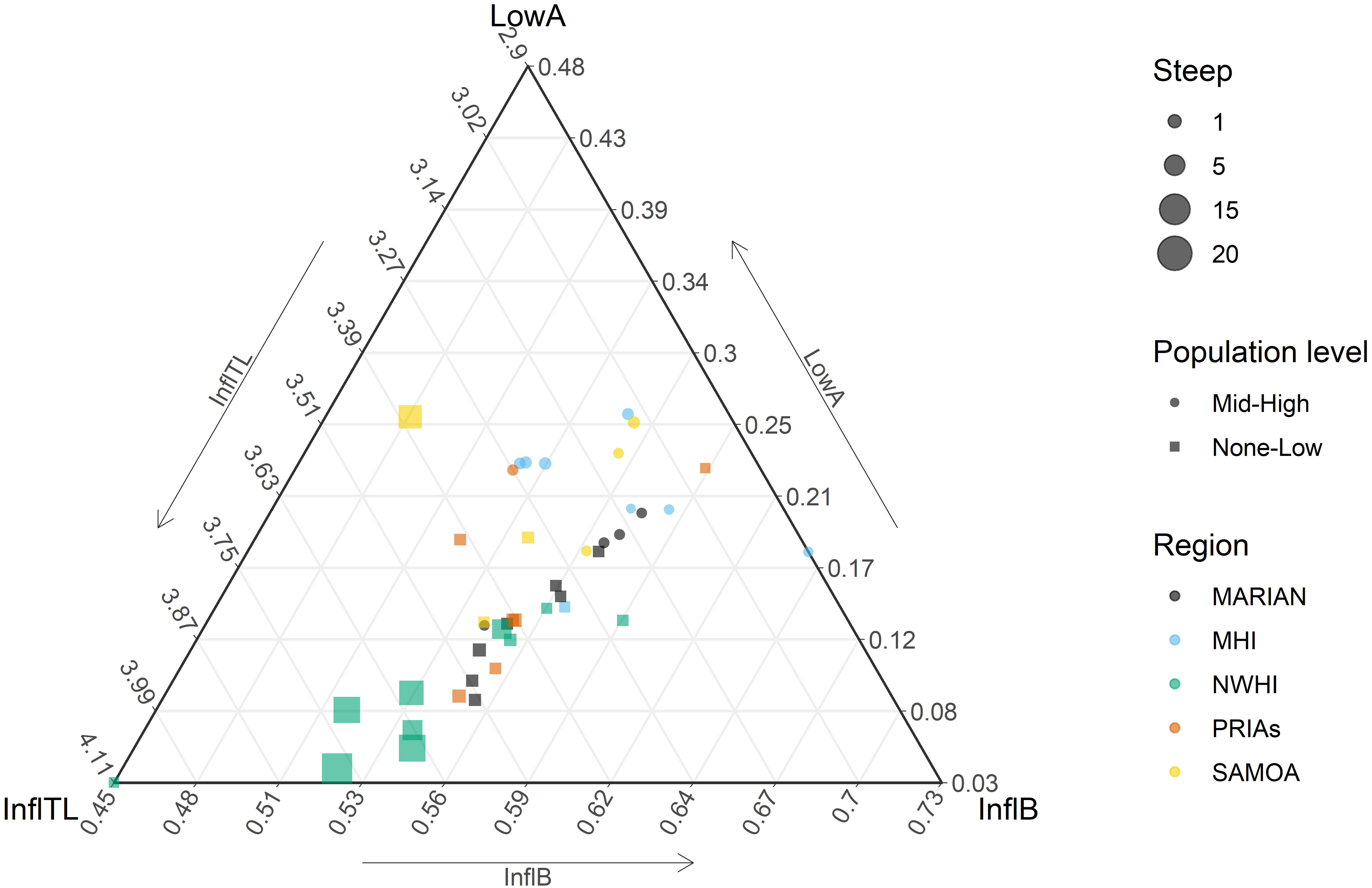
Figure 4 Ternary plot of three parameters (lower asymptote - LowA; %biomass at the inflection point - InflB; and TL of the inflection point; InflTL) of the cumulative biomass across trophic level curve. The size of the symbols (squares or circles, as shown in the scale) is proportional to the steepness (Steep); Marian, Mariana Archipelago; MHI, Main Hawaiian islands; NWHI, Northwestern Hawaiian Islands; PRIAs, Pacific Remote Island Areas; Samoa, American Samoa.

Examining the S-curve parameters shows that the less populated islands indeed had a higher inflection point TL and steepness across a range of biomass inflection point values, whereas higher populated islands have a higher LowA and lower InflTL and Steep. These would imply from cumulative trophic theory that a stronger perturbation is occurring in coral reefs at islands with higher human populations. There also appears to be consistency in S-curve parameters within an archipelago (Figures 4, 3), especially as seen in the Northwestern Hawaiian Islands curve parameters.

These distinctions across archipelago hold when examining them relative to various indicators of environmental conditions (Figure 5). The ordination shows a good separation among the different regions, except for the PRIAs, which overlapped with Samoan islands and partly with the Mariana Archipelago. The Northwestern Hawaiian Islands versus the Samoan and Pacific Remote Islands are on opposite sides of the first main multivariate axis, largely associated with wave height and variability of several environmental indicators on the left versus chlorophyl, temperature, and coral benthic coverage on the right. The secondary multivariate axis is less clear, though the main Hawaiian Islands have higher scores, which are loosely associated with higher hard bottom habitats and human populations. Collectively the PCA results imply that not all tropical islands in the Pacific share the same ambient features. The first two axes of the principal component analysis explained 54% of the total variance (Figure 5), with the first principal component mostly driven by island oceanographic characteristics and coral reef status, specifically wave energy (negatively), sea surface temperature (SST), irradiance and benthic substrate ratio (BSR) (positively). The second principal component can be interpreted as a human pressure gradient and associated coral reef status, driven mainly by human population variables and BSR, negatively related to the BSR index (positively related with the biomass of herbivorous fishes). Elucidating that not all islands in differing archipelagoes experience the same broader oceanographic context is elementary, but not trivial.

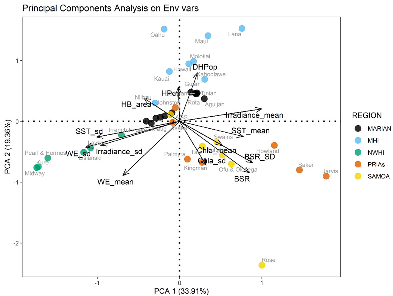
Figure 5 Biplot of the PCA on the mean environmental conditions and human pressures values. For variable labels see Table 2; Marian, Mariana Archipelago; MHI, Main Hawaiian islands; NWHI, Northwestern Hawaiian Islands; PRIAs, Pacific Remote Island Areas; Samoa, American Samoa.

When exploring the relationships of S-curve parameters across reefs from different islands with other measures of reef fish assemblage status, a few interesting observations arise (Figure 6). The observation that there are similar conditions within archipelagoes persists. As does the observation that generally exhibits different responses which contrast high human population with oceanic and reef conditions. What also emerges is that lower irradiance (i.e., less water clarity), higher human population, and lower coral cover are associated with curve parameters indicative of perturbation (higher LowA and lower InflTL and lower steepness), similar to Figure 3. But interestingly these situations are also associated with lower overall biomass, less biomass in upper trophic levels, and more biomass apportioned to lower TLs. There also appear to be a higher number of species in conditions with lower human population (Figure 6). The redundancy analysis shows that about 50% of the total variance of the assemblage indicators and the S-curve parameters can be explained in terms of environmental characteristics and human pressures.

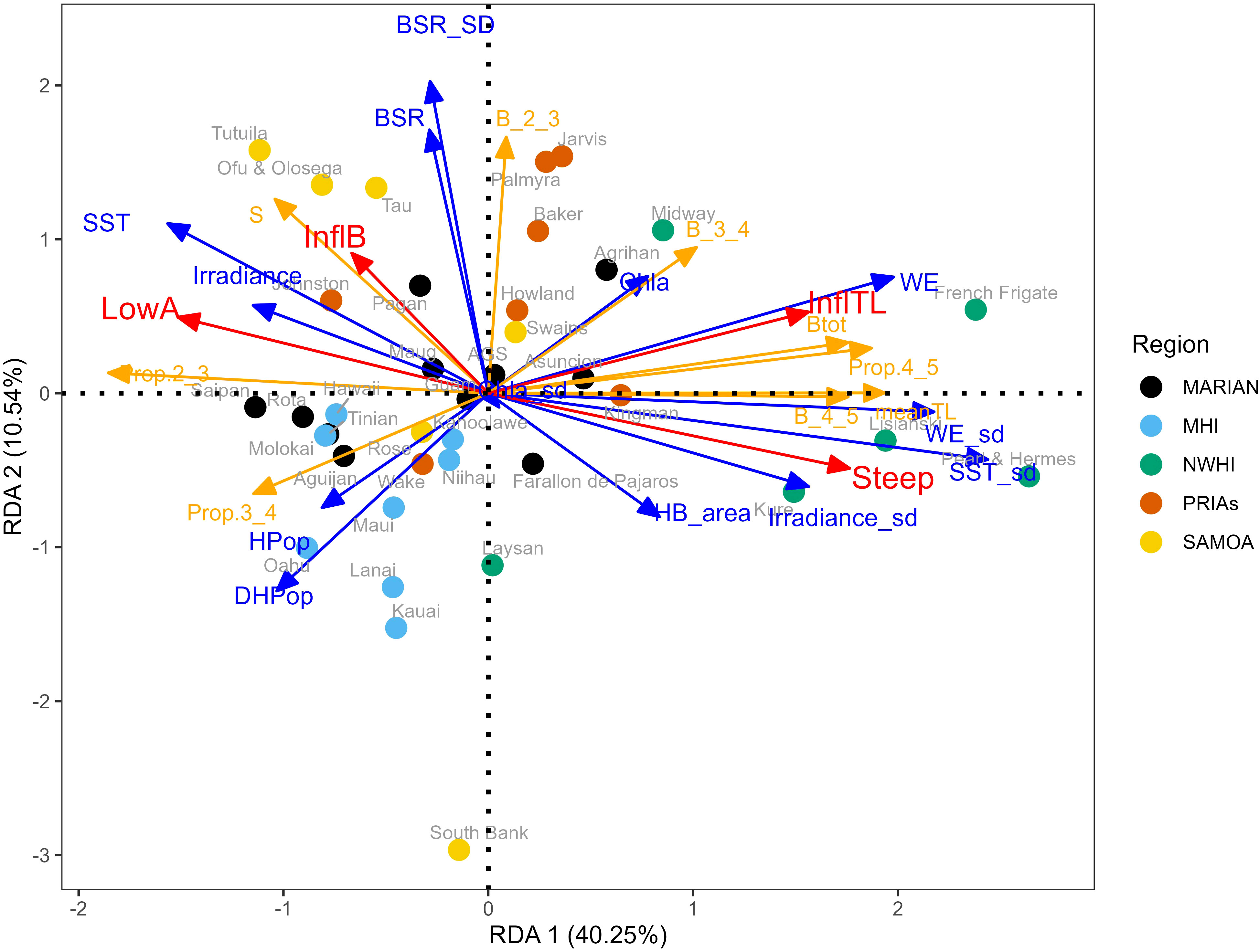
Figure 6 Triplot of the RDA. The blue arrows represent the mean environmental conditions and human pressure variables (for labels see Table 2), the red arrows represent the parameters of the curves (LowA=lower asymptote:; InflB=inflection biomass; InflTL=inflection; Steep=steepness), and the orange arrows represent the assemblage indicators (S: number species; Btot: total biomass; meanTL: mean trophic level, B_2_3: biomass between TL 2 and 3; Prop.2_3: proportion of the total biomass between TL 2 and 3; B_3_4: biomass between TL 3 and 4; Prop.3_4: proportion of the total biomass between TL 3 and 4; B_3_4: biomass between TL 4 and 5; Prop.4_5: proportion of the total biomass between TL 4 and 5) Marian, Mariana Archipelago; MHI, Main Hawaiian islands; NWHI, Northwestern Hawaiian Islands; PRIAs, Pacific Remote Island Areas; Samoa, American Samoa.

More clarity emerges when examining the bivariate relationship among S-curve parameters and assemblage indicators (Figure 7). The meanTL and total biomass were associated with higher steepness and InflTL values and lower LowA values as these values increased. The biomass at upper TLs also corresponded to higher steepness and InflTL and lower Low A values, similar to meanTL and total biomass. The proportion of biomass at TL4-5 showed opposition patterns to the lower TL biomass proportions, with lower TL biomass values associated with curve parameter values associated with more perturbed situations. These lower TL values tended to exhibit less variable relationships to the curve parameters. The number of species was intriguing, with less obvious patterns than the other assemblage metrics. Higher numbers of species were associated with higher values of LowA. This implies that the number of species may have helped to establish the lower curve intercept. No clear patterns emerged across the archipelagoes, as they were dispersed across both the range of curve parameters and assemblage metrics.

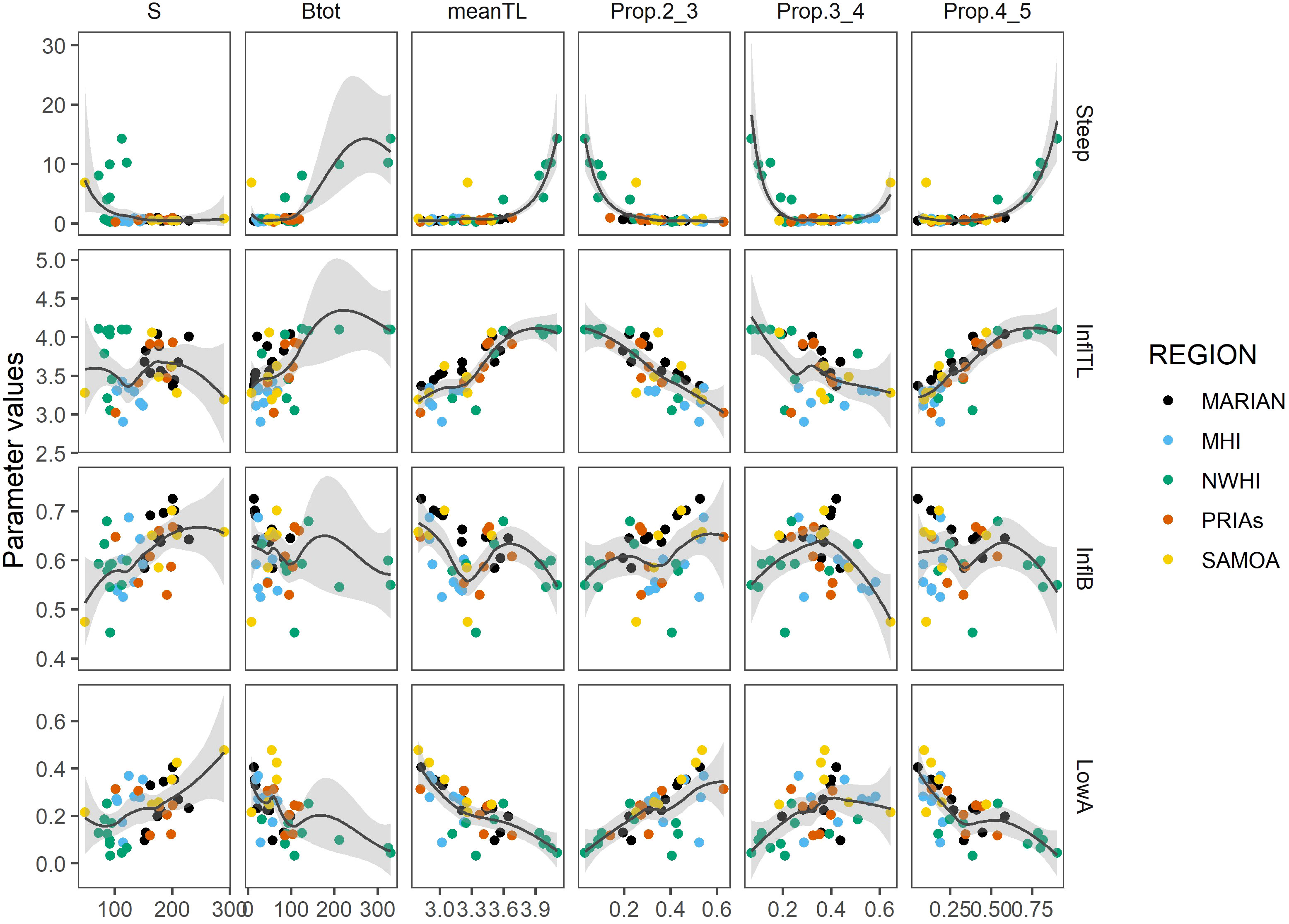
Figure 7 Relation between the parameters of the curves (LowA=lower asymptote:; InflB=inflection biomass; InflTL=inflection; Steep=steepness) and the assemblage indicators (S: number species; Btot: total biomass; meanTL: mean trophic level, Prop.2_3: proportion of the total biomass between TL 2 and 3; Prop.3_4: proportion of the total biomass between TL 3 and 4; Prop.4_5: proportion of the total biomass between TL 4 and 5).

When directly comparing the parameters of the curves between the scarcely populated and the highly populated islands, the LowA and InflTL seem to be able to best distinguish between the two groups (Figure 8). This is consistent with what would be expected in S-curve parameters, with human population a proxy for disturbance or perturbation. In this case, the response for steepness is primarily due to the presence of very steep curves for the Northwestern Hawaiian Islands, so that may or may not be indicative of a true relationship. That the InflB is more variable is not surprising given how S-curve shapes can vary and the underlying data used here. These results confirm and more clearly show the patterns in relation to human population seen in Figures 3-5. Again, as in the previous analyses, it is noteworthy that generally the observed pattern also holds when removing jacks and sharks (Supplementary Figures S2-S5). These latter two analyses imply that the interplay between island environmental features and human population can influence reef ecosystems to the same level of magnitude.

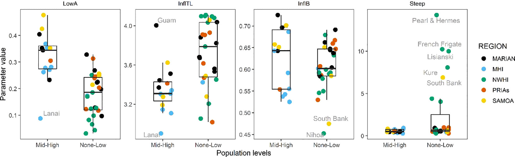
Figure 8 Boxplots for the parameters of the curves comparing the islands with different human population levels (none-low vs mid-high). LowA, lower asymptote; InflB, inflection biomass; InflTL, inflection; Steep, steepness; Marian, Mariana Archipelago; MHI, Main Hawaiian islands; NWHI, Northwestern Hawaiian Islands; PRIAs, Pacific Remote Island Areas; Samoa, American Samoa.

4 Discussion

Our results across many Pacific reef ecosystems adhere to expected global patterns from cumulative trophic theory (Link et al., 2015). In particular, the cumulative biomass-trophic level curves result in S-curves which are consistent and commonly observed from a range of marine ecosystems, including open ocean, upwelling, continental shelf, and estuarine ecosystems. They also respond to known pressures in a manner that is expected from cumulative trophic theory. This is both novel and not trivial, in large part because we were not sure if these patterns would be expressed in coral reefs ecosystems due to their unique biogenic habitat structure and differential food webs relative to other marine food webs. The salient point is that although there are distinctive facets of coral reef ecosystems, they confirm the global patterns (i.e., S-curves) expected from cumulative trophic theory.

Moreover, the cumulative curve approach was able to capture well the structure of the fish assemblages in coral reef ecosystems, as confirmed by the analysis contrasting the curve parameters with the fish assemblage metrics. In particular, the curve shape offers information not only about the biomass structure, but also about aspects of biodiversity, with some parameters positively related to the number of species. The relation between LowA and TL 2_3 biomass was expected, but the relation between InflB and number of species was rather unexpected as was the relationship between the steepness and total biomass. This implies that there are functional, structural, and energy flow dynamics that remain to be explored. It also confirms that the cumulative biomass approach can offer a synthetic picture of complex structures such as those in these coral reef ecosystems.

The multivariate relationships show two major patterns for these coral reefs. First is the dimension that highlights environmental gradients. Second is the dimension that notes the degree of pressures facing these coral reef ecosystems. The main features driving these patterns are indicative of the distinctions for each island reef ecosystem. There are obviously different oceanographic and habitat features that influence each broad region and these archipelagoes also experience an observable gradient of human pressures (Gove et al., 2013). The explainable variance in these analyses is moderate, implying both that these results have teased out some of the major distinctions in cumulative biomass curves for trophic coral reefs and that further features remain to be elucidated. However, it is reasonable to expect that not all the variability could be explained by the characterization carried out at the island scale, missing all (environmental, human pressures and fish biomass) of the variability within each island, and omitting relevant environmental variables and human impacts (Morais et al., 2020; Schiettekatte et al., 2022) which are not available at the temporal-spatial scale of this study. Both the PCA and the RDA analysis suggest that a composite view of these ecosystem emergent properties (considering the curve parameters) is more complicated (i.e., not completely explained by) than the one rising from just the environmental parameters; conversely, it confirms that the four curve parameters give slightly different information about the main drivers affecting the system, with the TL at the inflection point and steepness of the curves being the most affected by anthropogenic disturbances, and the other curve parameters (InflB point and LowA) also notably affected by environmental factors.

There are also distinctions across and within geographical regions in the Pacific. These may reflect latitudinal gradients across the archipelagoes, at least with respect to the surrounding oceanographic conditions (Williams et al., 2015; Heenan et al., 2020). Reporting and noting the cross-Archipelago differences exhibits two major patterns. The Marianas, Samoan, and Pacific Remote Islands experience relatively warmer temperatures and lower wave impacts, opposite of the Northwestern and Main Hawaiian Islands. There are implications to this, but this is also related to both Hawaiian Island chains tending to have lower inflection points for biomass and TL. Those patterns are then mitigated by human pressures.

It follows that a major pattern is observed for the US Pacific Island ecosystems that distinguishes coral reefs under pressure versus those that are not, largely proxied by human population density. The cumulative curve parameters are consistent with what one would expect for different levels of perturbation, with the areas more densely inhabited showing less pronounced S-curves. This is generally confirmed with other measures of reef status (benthic substrate ratio, reef fish assemblage metrics) whereby the S-curve is compressed towards the origin (Link et al., 2015). All this is reflected in the curve parameters, particularly inflection point of the TL and LowA, that discriminate well between the two groups (no/low inhabited vs mid/high inhabited). Human density was negatively related to the InflTL and positively to the LowA. All this agrees with the state of the reefs, which decreases with increasing human pressures (again, as also noted by the BSR index), producing an increase of herbivorous fish, with lower TL. Even without a clear distinction of the two groups, the steepness showed this generally negative response to both natural and anthropogenic disturbances. Remote islands showed the highest values of this parameter, implying a higher transfer efficiency to maintain high biomass of top predators (e.g., jacks and sharks), which would be seen in the steepness being able to transfer energy to upper TLs more rapidly, and as seen in InflTL and LowA, as having a larger basal part of the food web to support these apex predators.

As a corollary, the prior observation regarding top predators suggests an important role of energy exporting from the reef towards to open ocean, mediated by highly mobile species (Stevenson et al., 2007; Skinner et al., 2021). On the contrary, in more disturbed areas we observed an increase of the lower intercept, highlighting an increasing contribution of herbivorous species. This is probably due to an increase in internal energy utilization. This pattern could occur due to our curve-fitting method (fixing the maximum of the curve at 1), where a change in the upper part curve shape would be expected to produce a resetting of the lower part. But this is actually the mechanism we describe via these cumulative biomass-TL curves— that is, modification or adaptation of the curve shape in response to changing external drivers, leading to a larger fraction of energy stored in the lower TLs. From an ecological point of view this could represent an adaptation by the fish community where the reduced energy required by the higher TLs produced makes more energy available for the lower TLs, which increases fish biomass at those TLs. Thus, although this pattern could partially be an artefact of our fitting methodology, it could also represent legitimate dynamics more unique to coral reef ecosystems. Further examination of how energy is circulated in reef food webs relative to this pattern is warranted.

A novel metric produced in this work is the 4th curve parameter, the lower intercept (LowA), which is the point of interception of the curve on the y-axis. A key addition to the parameter set of these cumulative biomass-TL curves, it denotes the fish biomass of the low TL groups of species (particularly herbivores). This is why it was not emphasized, estimated, or was excluded in previous analyses that were based on fisheries landings (Libralato et al., 2019; Pranovi et al., 2020), since fisheries usually do not target lower TLs, even though they are well represented in the fish surveys used in some prior and certainly the present work. This parameter appears positively associated to anthropogenic pressure (population dimension), chl a, and SST, emphasizing the increase in terms of relative biomass of the herbivorous species under these more stressed conditions, perhaps due to increasing resource levels of algae as the condition of corals decrease on reefs. In terms of functional groups of herbivorous fishes, overall herbivore biomass decreases with increasing human population density, while SST has opposing effects on detritivores (positive) and browsers (negative) (Heenan et al., 2016), while the proportional biomass of these lower trophic level fishes increases in areas of high irradiance (Heenan et al., 2020). In essence, many of these herbivorous fish are primary targets of fishing in this region (Taylor, 2019), implying that the longer-term persistence of these fish is less likely with additional impact of habitat degradation and loss of reef structure, which makes such fish increasingly vulnerable to predation. A flattening of the S-curve and particularly lowering of LowA would detect such pressures. Hence, some of these archipelagoes expressing such patterns may be in an early phase of perturbation. This could indicate that the S-curve parameters are able to capture variations in trophic structure apparent in coral and macroalgal dominated reefs due to variable environmental drivers, if the presence of these fishes track their preferred resource and the signal is still apparent even in the presence of human pressures.

The use of emergent properties at the ecosystem level offers the opportunity for disclosing new perspectives in the analysis of the ecological processes and functioning of marine ecosystems. It is often difficult and quite involved to fully and quickly grasp the status of these reefs in their entirety as a full system (Fenner, 2012; Boyle et al., 2017; Obura et al., 2019); perhaps the S-curve parameters presented here, which tend to track and confirm known responses of coral reefs to known pressures (Williams et al., 2015; Heenan et al., 2016; Gorospe et al., 2018; Heenan et al., 2020), could be another way to provide a relatively quick overview of coral reef status. Thus, we propose the suite of metrics and measures presented herein as an integrated suite of metrics for the examination of coral reef ecosystem functioning, and to delineate their status and the relative degree of perturbation (or recovery) that a reef may be experiencing. The cumulative biomass curve approach allows us to directly combine biomass (a parameter describing the ecosystem structure) with the energy transfer across TLs (describing key aspects the ecosystem functioning and structure) to elucidate a clearer and different perspective of coral reefs. Moreover, this approach can be useful for analyzing time series data in one place over time, in relation to disturbance events, to see how effective it is in tracking food web response and recovery as has been done in studies of other ecosystems (Pranovi et al., 2014; Libralato et al., 2019; Pranovi et al., 2020).

We posit that cumB-TL curves are in fact now global, as everywhere and every time they have been examined for marine ecosystems, we see these patterns repeated. The cumulative trophic theory (Link et al., 2015; Libralato et al., 2019) has become increasingly robust with each new additional study, as caveats and novel, even if subtle (e.g., the lower intercept parameter here) additions to our understanding of how ecosystems accumulate and distribute biomass, production and energy continue to accumulate. We assert that the outcomes from cumulative theory can begin to be codified into operational, management contexts. And importantly, this now includes tropical coral reef ecosystems.

Data availability statement

The original contributions presented in the study are included in the article/Supplementary Material, further inquiries can be directed to the corresponding author.

Author contributions

JL: Conceptualization, Project administration, Writing – original draft, Writing – review & editing. FP: Conceptualization, Methodology, Project administration, Writing – original draft. MZ: Conceptualization, Formal Analysis, Methodology, Software, Writing – review & editing. TK: Data curation, Writing – review & editing. AH: Data curation, Writing – review & editing. KT: Data curation, Writing – review & editing.

Funding

The author(s) declare financial support was received for the research, authorship, and/or publication of this article. The NCRMP surveys were funded by the NOAA Coral Reef Conservation Program project #743, and research cruises were conducted with additional support from the NOAA Pacific Islands Fisheries Science Center’s Ecosystem Sciences Division (PIFSC ESD), NOAA Ships Hi’ialakai and Oscar Elton Sette, and the partner agencies that contributed to field and survey operations and provided permission to work in local waters. NOAA and University of Venice provided funding for scientific exchanges for JL and FP.

Acknowledgments

We thank the NOAA NMFS PIFSC NCRMP staff and their associated partners for conducting cruises, processing samples, and maintaining these data. We thank Jennifer Dusto for her assistance in formatting the literature. We thank Courtney Couch and her team of annotators for calculating the benthic substrate ratios at the NCRMP sites. We thank Rusty Brainard, Erica Towle, Jay Grove, Jamie Gove, and reviewers for their comments on previous versions of the manuscript. We want to particularly note that this work is the result of low‐key, long‐term, ongoing collaborations and it is not the result of huge programs or large, funded projects but simple, curiosity‐ and friendship‐based science. These latter forms of science are needed and we want to highlight them here as they seem to be at risk of being lost or at least certainly becoming less frequent. We also note the benefit of investing in scientific exchanges and moderate travel to facilitate such interactions over the years. This work was ultimately initiated on a paper placemat at a restaurant in Venice nearly 15 years ago, and the resultant, continued development of this theory has stemmed from that original and subsequent (e.g. coffee at a beachside café in Honolulu), similar interactions.

Conflict of interest

The authors declare that the research was conducted in the absence of any commercial or financial relationships that could be construed as a potential conflict of interest.

Publisher’s note

All claims expressed in this article are solely those of the authors and do not necessarily represent those of their affiliated organizations, or those of the publisher, the editors and the reviewers. Any product that may be evaluated in this article, or claim that may be made by its manufacturer, is not guaranteed or endorsed by the publisher.

Supplementary material

The Supplementary Material for this article can be found online at: https://www.frontiersin.org/articles/10.3389/fmars.2023.1324053/full#supplementary-material

References

Baker A. C., Glynn P. W., Riegl B. (2008). Climate change and coral reef bleaching: an ecological assessment of long-term impacts, recovery trends and future outlook. Estuarine Coast. Shelf Sci. 80, 435–471. doi: 10.1016/j.ecss.2008.09.003
Barbier E. B., Hacker S. D., Kennedy C., Koch E. W., Stier A. C., Silliman B. R. (2011). The value of estuarine and coastal ecosystem services. Ecol. Monogr. 81, 169–193. doi: 10.1890/10-1510.1
Becker J. J., Sandwell D. T., Smith W. H. F., Braud J., Binder B., Depner J., et al. (2009). Global bathymetry and elevation data at 30 arc seconds resolution: SRTM30_PLUS. Mar. Geodesy 32 (4), 355–371. doi: 10.1080/01490410903297766
Beijbom O., Edmunds P. J., Roelfsema C., Smith J., Kline D. I., Neal B. P., et al. (2015). Towards automated annotation of benthic survey images: variability of human experts and operational modes of automation. PloS One 10 (7), e0130312. doi: 10.1371/journal.pone.0130312
Bellwood D. R., Streit R. P., Brandl S. J., Tebbett S. B. (2019). The meaning of the term ‘function’in ecology: A coral reef perspective. Funct. Ecol. 33 (6), 948–961. doi: 10.1111/1365-2435.13265
Boyle S., De Anda V., Koenig K., O’Reilly E., Schafer M., Acoba T., et al. (2017). Coral reef ecosystems of the Pacific Remote Islands Marine National Monument: a 2000– 2016 overview (Honolulu, HI: NOAA PIFSC Special Publication, SP-17-003), 62.
Brainard R. E., Acoba T., Asher M. A. M., Asher J. M., Ayotte P. M., Barkley H. C., et al. (2019). “Pacific Remote Islands Marine National Monument in the Pacific-wide Context,” in Coral Reef Ecosystem Monitoring Report for the Pacific Remote Islands Marine National Monument 2000–2017, vol. SP-19-006i. (Honolulu: Pacific Islands Fisheries Science Center, PIFSC Special Publication), 72. doi: 10.25923/rwd2-2118
Brainard R. E., Asher J., Blyth-Skyrme V., Coccgna E. F., Dennis K., Donovan M. K., et al. (2012). Coral reef Ecosystem Monitoring Report for the Mariana Archipelago: 2003 – 2007 (Honolulu: NOAA Fisheries, Pacific Islands Fisheries Science Center, PIFSC Special Publication, SP-12-01), 1019.
Brewer T. D., Cinner J. E., Green A., Pressey R. L. (2013). Effects of human population density and proximity to markets on coral reef fishes vulnerable to extinction by fishing. Conserv. Biol. 27 (3), 443–452. doi: 10.1111/j.1523-1739.2012.01963.x
Burke L., Reytar K., Spalding M., Perry A. (2011). Reefs at risk revisited (Washington, D.C: World Resources Institute).
Cinner J. (2014). Coral reef livelihoods. Curr. Opin. Environ. Sustainability 7, 65–71. doi: 10.1016/j.cosust.2013.11.025
Cinner J. E., Graham N. A., Huchery C., MacNeil M. A. (2013). Global effects of local human population density and distance to markets on the condition of coral reef fisheries. Conserv. Biol. 27 (3), 453–458. doi: 10.1111/j.1523-1739.2012.01933.x
Cinner J. E., Huchery C., MacNeil M. A., Graham N. A., McClanahan T. R., Maina J., et al. (2016). Bright spots among the world’s coral reefs. Nature 535, 416–419. doi: 10.1038/nature18607
de Young B., Heath M., Werner F., Chai F., Megrey B., Monfray P. (2004). Challenges of modeling ocean basin ecosystems. Science 304, 1463–1466. doi: 10.1126/science.1094858
Dubinsky Z., Stambler N. (1996). Marine pollution and coral reefs. Global Change Biol. 2, 511–526. doi: 10.1111/j.1365-2486.1996.tb00064.x
Erftemeijer P. L. A., Riegl B., Hoeksema B. W., Todd P. A. (2012). Environmental impacts of dredging and other sediment disturbances on corals: a review. Mar. pollut. Bull. 64, 1737–1765. doi: 10.1016/j.marpolbul.2012.05.008
Fabricius K. E. (2005). Effects of terrestrial runoff on the ecology of corals and coral reefs: review and synthesis. Mar. pollut. Bull. 50, 125–146. doi: 10.1016/j.marpolbul.2004.11.028
Fenner D. (2012). Challenges for managing fisheries on diverse coral reefs. Diversity 4, 105–160. doi: 10.3390/d4010105
Froese R., Pauly D. Editors. (2023). FishBase. World Wide Web electronic publication. Available at: https://www.fishbase.org, version (10/2023).
Gorospe K. D., Donahue M. J., Heenan A., Gove J. M., Williams I. D., Brainard R. E. (2018). Local biomass baselines and the recovery potential for Hawaiian coral reef fish communities. Front. Mar. Sci. 5, 162. doi: 10.3389/fmars.2018.00162
Gove J. M., Williams G. J., McManus M. A., Heron S. F., Sandin S. A., Vetter O. J. (2013). Quantifying climatological ranges and anomalies for pacific coral reef ecosystems. PloS One 8 (4), e61974. doi: 10.1371/journal.pone.0061974
Harfoot M. B. J., Newbold T., Tittensor D. P., Emmott S., Hutton J., Lyutsareev V., et al. (2014). Emergent global patterns of ecosystem structure and function from a mechanistic general ecosystem model. PloS Biol. 12 (4), e1001841. doi: 10.1371/journal.pbio.1001841
Heenan A., Asher J. M., Ayotte P., Gorospe K., Giuseffi L., Gray A., et al. (2018). Pacific reef assessment and monitoring program. Fish Monit. brief: Jarvis Island time Trends, DR–18-003. doi: 10.7289/V5/DR-PIFSC-18-003
Heenan A., Hoey A. S., Williams G. J., Williams I. D. (2016). Natural bounds on herbivorous coral reef fishes. Proc. R. Soc B Biol. Sci. 283, 1716. doi: 10.1098/rspb.2016.1716
Heenan A., Williams G. J., Williams I. D. (2020). Natural variation in coral reef trophic structure across environmental gradients. Front. Ecol. Environ. 18 (2), 69–75. doi: 10.1002/fee.2144
Heron S. F., Maynard J. A., Van Hooidonk R., Eakin C. M. (2016). Warming trends and bleaching stress of the world’s coral reefs 1985-2012. Sci. Rep. 6, 38402. doi: 10.1038/srep38402
Hoegh-Guldberg O. (1999). Climate change, coral bleaching and the future of the world’s coral reefs. Mar. Freshw. Res. 50, 839–866. doi: 10.1071/mf99078
Hoegh-Guldberg O., Poloczanska E. S., Skirving W., Dove S. (2017). Coral reef ecosystems under climate change and ocean acidification. Front. Mar. Sci. 4. doi: 10.3389/fmars.2017.00158
Houk P., Benavente D., Iguel J., Johnson S., Okano R. (2014). Coral reef disturbance and recovery dynamics differ across gradients of localized stressors in the mariana islands. PloS One 9 (8), e105731. doi: 10.1371/journal.pone.0105731
Houk P., Musburger C., Wiles P. (2010). Water quality and herbivory interactively drive coral-reef recovery patterns in american Samoa. PloS One 5 (11), e13913. doi: 10.1371/journal.pone.0013913
Hughes T. P., Anderson K. D., Connolly S. R., Heron S. F., Kerry J. T., Lough J. M., et al. (2018). Spatial and temporal patterns of mass bleaching of corals in the Anthropocene. Science 359, 80–83. doi: 10.1126/science.aan8048
Hughes T. P., Baird A. H., Bellwood D. R., Card M., Connolly S. R., Folke C., et al. (2003). Climate change, human impacts, and the resilience of coral reefs. Science 301, 929–933. doi: 10.1126/science.1085046
Hughes T. P., Bellwood D. R., Connolly S. R. (2002). Biodiversity hotspots, centres of endemicity, and the conservation of coral reefs. Ecol. Lett. 5, 775–784. doi: 10.1046/j.1461-0248.2002.00383.x
Jackson J. B. C., Kirby M. X., Berger W. H., Bjorndal K. A., Botsford L. W., Bourque B. J., et al. (2001). Historical overfishing and the recent collapse of coastal ecosystems. Science 293, 629–638. doi: 10.1126/science.1059199
Kulbicki M., Guillemot N., Amand M. (2005). A general approach to length-weight relationships for New Caledonian lagoon fishes. Cybium 29 (3), 235–252.
Langdon C., Atkinson M. J. (2005). Effect of elevated pCO2 on photosynthesis and calcification of corals and interactions with seasonal change in temperature/irradiance and nutrient enrichment. J. Geophys. Res. 110, C09S07. doi: 10.1029/2004JC002576
Libralato S., Pranovi F., Zucchetta M., Monti M. A., Link J. S. (2019). Global thresholds in properties emerging from cumulative curves of marine ecosystems. Ecol. Indic. 103, 554–562. doi: 10.1016/j.ecolind.2019.03.053
Link J. S., Pranovi F., Libralato S., Coll M., Christensen V., Solidoro C., et al. (2015). Emergent properties delineate marine ecosystem perturbation and recovery. Trends Ecol. Evol. 30, 649–661. doi: 10.1016/j.tree.2015.08.011
Link J. S., Watson R. A., Pranovi F., Libralato S. (2020). Comparative production of fisheries yields and ecosystem overfishing in African Large Marine Ecosystems. Environ. Dev. 36. doi: 10.1016/j.envdev.2020.100529
Maire E., Cinner J., Velez L., Huchery C., Mora C., Dagata S., et al. (2016). How accessible are coral reefs to people? A global assessment based on travel time. Ecol. Lett. 19 (4), 351–360. doi: 10.1111/ele.12577
McCoy K., Asher J. M., Ayotte P., Gray A. K., Kindinger T., Williams I. (2019). Pacific Reef Assessment and Monitoring Program Data Report Ecological monitoring 2019—Reef fishes and benthic habitats of the main Hawaiian Islands. PIFSC Data Rep. DR-19-039., 35 p. doi: 10.25923/he4m-6n68
Moberg F., Folke C. (1999). Ecological goods and services of coral reef ecosystems. Ecol. Economics 29, 215–233. doi: 10.1016/s0921-8009(99)00009-9
Morais R. A., Depczynski M., Fulton C., Marnane M., Narvaez P., Huertas V., et al. (2020). Severe coral loss shifts energetic dynamics on a coral reef. Funct. Ecol. 34, 1507–1518. doi: 10.1111/1365-2435.13568
Mouillot D., Villéger S., Parravicini V., Kulbicki M., Arias-González J. E., Bender M., et al. (2014). Functional over-redundancy and high functional vulnerability in global fish faunas on tropical reefs. Proc. Natl. Acad. Sci. 111 (38), 13757–13762. doi: 10.1073/pnas.1317625111
Newton K., Côté I. M., Pilling G. M., Jennings S., Dulvy N. K. (2007). Current and future sustainability of island coral reef fisheries. Curr. Biol. 17, 655–658. doi: 10.1016/j.cub.2007.02.054
Obura D. O., Aeby G., Amornthammarong N., Appeltans W., Bax N., Bishop J., et al. (2019). Coral reef monitoring, reef assessment technologies, and ecosystem-based management. Front. Mar. Sci. 6. doi: 10.3389/fmars.2019.00580
Oksanen J., Blanchet F. G., Friendly M., Kindt R., Legendre P., McGlinn D., et al. (2020). Vegan: Community Ecology Package. Available at: https://CRAN.R-project.org/package=vegan.
Pandolfi J. M., Connolly S. R., Marshall D. J., Cohen A. L. (2011). Projecting coral reef futures under global warming and ocean acidification. Science 333, 418–422. doi: 10.1126/science.1204794
Pranovi F., Libralato S., Zucchetta M., Link J. (2014). Biomass accumulation across trophic levels: analysis of landings for the Mediterranean Sea. Mar. Ecol. Prog. Ser. 512, 201–216. doi: 10.3354/meps10881
Pranovi F., Libralato S., Zucchetta M., Monti M. A., Link J. S. (2020). Cumulative biomass curves describe past and present conditions of Large Marine Ecosystems. Global Change Biol. 26, 786–797. doi: 10.1111/gcb.14827
Pranovi F., Link J. S. (2009). Ecosystem exploitation and trophodynamic indicators: a comparison between the Northern Adriatic Sea and Southern New England. Prog. Oceanography 81, 149–164. doi: 10.1016/j.pocean.2009.04.008
Pranovi F., Link J., Fu C., Cook A. M., Liu H., Gaichas S., et al. (2012). Trophic-level determinants of biomass accumulation in marine ecosystems. Mar. Ecol. Prog. Ser. 459, 185–201. doi: 10.3354/meps09738
Reaka-Kudla M. L. (1997). “The global biodiversity of coral reefs: a comparison with rain forests,” in Diversity II: understanding and protecting our biological resources (Washington, D.C: Joseph Henry Press), 83–108.
R Core Team. (2021). R: A language and environment for statistical computing. Published online 2020. Supplemental Information References S, 1, 371–378.
Richardson L. E., Graham N. A. J., Pratchett M. S., Eurich J. G., Hoey A. S. (2018). Mass coral bleaching causes biotic homogenization of reef fish assemblages. Global Change Biol. 24, 3117–3129. doi: 10.1111/gcb.14119
Ricketts J. H., Head G. A. (1999). A five-parameter logistic equation for investigating asymmetry of curvature in baroreflex studies. Am. J. Physiology-Regulative Integrat. Comparat. Physiol. 277 (3), R441–R454. doi: 10.1152/ajpregu.1999.277.2.R441
Ritz C., Baty F., Steibig J. C., Gerhard D. (2015). Dose-response analysis using R. PloS One 10 (12), e0146021. doi: 10.1371/journal.pone.0146021
Robinson J. P., Williams I. D., Edwards A. M., McPherson J., Yeager L., Vigliola L., et al. (2017). Fishing degrades size structure of coral reef fish communities. Glob. Change Biol. 23, 1009–1022. doi: 10.1111/gcb.13482
Rogers C. S. (1990). Responses of coral reefs and reef organisms to sedimentation. Mar. Ecol. Prog. Ser. 62, 185–202. doi: 10.3354/meps062185
Schiettekatte N. M. D., Brandl S. J., Casey J. M., Graham N. A. J., Barneche D. R., Burkepile D. E., et al. (2022). Biological trade-offs underpin coral reef ecosystem functioning. Nat. Ecol. Evol. 6, 701–708. doi: 10.1038/s41559-022-01710-5
Skinner C., Mill A. C., Fox M. D., Newman S. P., Zhu Y., Kuhl A., et al. (2021). Offshore pelagic subsidies dominate carbon inputs to coral reef predators. Sci. Adv. 7, eabf3792. doi: 10.1126/sciadv.abf3792
Steele J. H. (1985). A comparison of terrestrial and marine ecological systems. Nature 313, 355–358.
Stevenson C., Katz L. S., Micheli F., Block B., Heiman K. W., Perle C., et al. (2007). High apex predator biomass on remote Pacific islands. Coral Reefs 26, 47–51. doi: 10.1007/s00338-006-0158-x
Taylor B. M. (2019). Standing out in a big crowd: high cultural and economic value of naso unicornis in the insular pacific. Fishes 4 (3), 40. doi: 10.3390/fishes4030040
Williams I. D., Baum J. K., Heenan A., Hanson K. M., Nadon M. O., Brainard R. E. (2015). Human, oceanographic and habitat drivers of central and western pacific coral reef fish assemblages. PloS One 10, e0120516. doi: 10.1371/journal.pone.0120516
Williams I. D., Couch C. S., Beijbom O., Oliver T. A., Vargas-Angel B., Schumacher B. D., et al. (2019). Leveraging automated image analysis tools to transform our capacity to assess status and trends of coral reefs. Front. Mar. Sci. 6. doi: 10.3389/fmars.2019.00222
Keywords: emergent properties, cumulative biomass, fish community biomass, tropical ecosystems, island reefs, perturbations, ecosystem recovery, trophic level
Citation: Link JS, Pranovi F, Zucchetta M, Kindinger TL, Heenan A and Tanaka KR (2024) Cumulative trophic curves elucidate tropical coral reef ecosystems. Front. Mar. Sci. 10:1324053. doi: 10.3389/fmars.2023.1324053
Received: 18 October 2023; Accepted: 13 December 2023;
Published: 04 January 2024.
Edited by:
Michelle Jillian Devlin, Centre for Environment, Fisheries and Aquaculture Science (CEFAS), United KingdomReviewed by:
Luis Eduardo Calderon Aguilera, Center for Scientific Research and Higher Education in Ensenada (CICESE), MexicoDavid Chagaris, University of Florida, United States
Copyright © 2024 Link, Pranovi, Zucchetta, Kindinger, Heenan and Tanaka. This is an open-access article distributed under the terms of the Creative Commons Attribution License (CC BY). The use, distribution or reproduction in other forums is permitted, provided the original author(s) and the copyright owner(s) are credited and that the original publication in this journal is cited, in accordance with accepted academic practice. No use, distribution or reproduction is permitted which does not comply with these terms.
*Correspondence: Jason S. Link, Jason.Link@noaa.gov