
Alteration Detection of Multispectral/Hyperspectral Images Using Dual-Path Partial Recurrent Networks


1
Faculty of Information Technology, Macau University of Science and Technology, Macau 853, China
2
School of Applied Sciences, Macao Polytechnic Institute, Macau 853, China
*
Author to whom correspondence should be addressed.
Remote Sens. 2021, 13(23), 4802; https://doi.org/10.3390/rs13234802
Submission received: 12 October 2021
/
Revised: 23 November 2021
/
Accepted: 23 November 2021
/
Published: 26 November 2021
(This article belongs to the Section Remote Sensing Image Processing)
Abstract
:Numerous alteration detection methods are designed based on image transformation algorithms and divergence of bi-temporal images. In the process of feature transformation, pseudo variant information caused by complex external factors will be highlighted. As a result, the error of divergence between the two images will be further enhanced. In this paper, we propose to fuse the variability of Deep Neural Networks’ (DNNs) structure flexibly with various detection algorithms for bi-temporal multispectral/hyperspectral imagery alteration detection. Specifically, the novel Dual-path Partial Recurrent Networks (D-PRNs) was proposed to project more accurate and effective deep features. The Unsupervised Slow Feature Analysis (USFA), Iteratively Reweighted Multivariate Alteration Detection (IRMAD), and Principal Component Analysis (PCA) were then utilized, respectively, with the proposed D-PRNs, to generate two groups of transformed features corresponding to the bi-temporal remote sensing images. We next employed the Chi-square distance to compute the divergence between two groups of transformed features and, thus, obtain the Alteration Intensity Map. Finally, threshold algorithms K-means and Otsu were, respectively, applied to transform the Alteration Intensity Map into Binary Alteration Map. Experiments were conducted on two bi-temporal remote sensing image datasets, and the testing results proved that the proposed alteration detection model using D-PRNs outperformed the state-of-the-art alteration detection model.
1. Introduction
Imagery alteration detection generally refers to the techniques of divergence recognition in the same geographical location observed over time in order to detect the pixel-level alterations caused by various natural and human factors, such as the alterations of river channels, geological disasters, artificial buildings, vegetation cover, and so on. The availability of open and shared bi-temporal multispectral/hyperspectral imagery datasets, as well as Synthetic Aperture Radar (SAR) imagery datasets, facilitates researchers in testing the superiority of proposals for alteration detection. Moreover, many imagery datasets are radiometric corrected [1,2,3,4], which offers a foundation for the following works such as image recognition [5,6,7], analysis, and classification [8,9]. Therefore, we can focus straightforwardly on constructing alteration detection models with good performance.
Generally, in the field of alteration detection, the widely used transformation algorithms have been proposed to extract and map the original image data into a new space. After that, the variant features will be highlighted to achieve greater contrast of the bi-temporal features. The transformation algorithms are mainly the classical Multivariate Alteration Detection (MAD) [10], which also serves other transformation algorithms, Iteratively Reweighted Multivariate Alteration Detection (IRMAD) [11] and the Principal Component Analysis (PCA) [12], as well as the Independent Component Analysis (ICA) [13] and the Gramm Schmidt (GS) [14]. However, in practice, the transformation algorithms are sometimes less effective in reducing the negative impact of noise. Therefore, in this paper, we propose to alleviate the problem by applying deep learning algorithms to detected images. Thus, pseudo features are effectively suppressed [1,2,15].
During the past several years, many methods have been proposed to apply DNNs for projecting essential deep features. [16,17,18,19,20,21,22,23,24]. Ghosh et al. [25] proposed to integrate semi-supervised learning with an improved, self-organizing feature, map-based, alteration detection technique and unsupervised context sensitivity. Zhang et al. [19] adopted an image fusion network with deep supervision for alteration detection in bi-temporal hyperspectral images. Connors et al. [26] presented a deep generative model-based method with Deep Rendering Mixture for alteration detection in very-high-resolution (VHR) images. Chen et al. [27] presented an advanced, Siamese, multilayered, convolutional, recurrent neural network (SiamCRNN) with wide applicability for alteration detection in multi-temporal and homogeneous/heterogeneous VHR images. Andermatt et al. [28] proposed a weakly supervised alteration detection network, W-CDNet, which receives the training samples with image-level semantic labels. Daudt et al. [29] specially designed a guided anisotropic diffusion (GAD) algorithm used as two strategies of weak supervision for alteration detection. Zhang et al. [30] proposed an excellent supervised alteration detection algorithm based on modified, triplet-state loss function for aerial images.
Although the abovementioned models have achieved very good alteration detection results, their defects and flaws are quite apparent. That is, they are based on complex and supervised network structures. The several shortcomings of them are as follows. First, in essence, supervised learning slightly deviates from the original intention of artificial intelligence to guide the fitting model. Second, the final detection results of approaches with supervised learning are related not only to the guidance mode of supervision signals but also to the distribution of artificial labels. However, generating appropriate labels is another challenge of supervision-based deep learning, and not properly solving may lead to the error description of effective features to a certain extent. Additionally, it is difficult to measure and protect the effective fitting model from being misguided. Third, whether to label the real scenes or the image data, it requires varying degrees of labor cost. In practical application, the images to be detected are not always annotated. Fourth, alteration detection models with supervised mode, as well as the complex deep network frameworks, are at a disadvantage in terms of time and resource consumption.
Accordingly, in this paper, we propose two symmetric, light-weight networks to serve our proposal, the Alteration Detection Model using Dual-path Partial Recurrent Networks (ADM-D-PRNs). The proposed ADM-D-PRNs have wide applicability in bi-temporal multispectral/hyperspectral imagery alteration detection. Experimental results showed that the ADM-D-PRNs achieved better detection results than the outstanding baselined Deep Slow Feature Analysis (DSFA) [31] series models on multispectral/hyperspectral dataset ‘Taizhou’/‘River’. In the proposed ADM-D-PRNs, the Change Vector Analysis (CVA) Binary Alteration Map provided a reference for DNNs to select invariant pixel pairs with high confidence as training samples. The proposed D-PRNs learned to suppress noise/pseudo features and project more accurate and effective features into a new space. Remarkably, the performance of alteration detection models based on pre-detection and DNNs was not only related to the suitability of a DNN but also to the confidence of training samples corresponding to the pixels in a pre-detected Binary Alteration Map. In the proposed ADM-D-PRNs, the three post-processing algorithms, Unsupervised Slow Feature Analysis (USFA), IRMAD, and PCA, w respectively employed to realize the mutual supplement and achieve the optimization of the essential bi-temporal features. Significantly, the quality of deep features has a crucial impact in the whole detection model; also, the action of post-processing algorithms on deep features with serious distortions will further amplify the erroneous description.
We organized the rest of this paper as follows. Section 2 presents the details of the proposed schema. Section 3 demonstrates and compares the experimental results of several alteration detection models. Section 4 discusses the specific results under different sampling strategies. In Section 5, we draw the conclusions and offer the future work.
2. Proposed ADM-D-PRNs
Figure 1 shows the flowchart of the proposed ADM-D-PRNs. Firstly, the CVA pre-detection method was employed to compute bi-temporal images and generate the CVA Binary Alteration Map, from which the invariant pixels with high confidence were extracted and, thus, selected as training samples. Then, the proposed D-PRNs was applied for learning the training samples and transforming the bi-temporal images into a new feature space for detection analysis and calculation. After that, different post-processing methods were employed. The USFA was used to suppress the invariant features and highlight the variant features, while the IRMAD and PCA were used to obtain the well-transformed description features by dimension reduction, thereby enhancing the effect on pixel classification. By applying the Chi-square distance, the Alteration Intensity Map could be calculated. Finally, the threshold algorithms, K-means [32] and Otsu [33], were respectively employed to generate the Binary Alteration Map.
2.1. CVA Pre-Detection
Generally, there are several strategies for the sample source in practice. In the proposed ADM-D-PRNs, we proposed to use invariant pixel pairs with high confidence to train the networks. We selected the invariant pixels randomly as training samples and, thus, achieved a better performance than the other sampling strategies. The metrics’ accuracy of a training model based on pre-detection mainly depends on two aspects: first, enough training samples and, second, training samples with high confidence. In summary, by learning the invariant pixels with high confidence, features with higher confidence can be obtained.
Considering that the input of the ADM-D-PRNs is pixel pairs from the bi-temporal multispectral/hyperspectral images, we firstly employed the CVA pre-detection method to generate the CVA Binary Alteration Map, from which the invariant pixels with high confidence were then generated as training samples.
As an extension of the simple divergence method in multispectral/hyperspectral images, CVA calculates the changing magnitude through an overall divergence operation of each pixel pair of bi-temporal images. As Equation (1) shows, the changing vector consists of the variation of each pixel pairs, considering all spectral bands. Then the CVA Alteration Intensity Map, CVA_AIM, can be obtained by applying the Euclidean Distance [34], as shown in Equation (2).
where D denotes the divergence of each spectral band pairs and consists of b vectors; b denotes the number of spectral bands; k denotes the band index with the range of values from 1 to b; i and j denote the pixel index in the image matrix, with the range of values from 0 to and from 0 to , where the r and c are the height and width of the current image in pixels; n represents the number of pixels in each image; the and represent the feature values in position (i, j) of two data matrices of the k-th spectral band.
2.2. The Proposed D-PRNs
Different from the common image recognition and detection tasks that process one image at a time, the alteration detection task processes at least two images at the same time, and the projection features must meet the needs of alteration detection. To fulfill the needs of the alteration detection task, we proposed the D-PRNs to project two groups of deep features, which better describe the divergence of the bi-temporal images. Figure 2 shows the structure of the proposed D-PRNs. In order to facilitate the process of D-PRNs, the image features are reshaped into vectors, each of which stores feature values of an image band. As Figure 2 shows, the red nodes in the leftmost input layer represent the pixel-wise features of each image band, and the number of red nodes in this layer is equivalent to the number of image bands. Similarly, the red nodes in the rightmost layer represent the output features. The second and third layers with 128 blue nodes are the two hidden layers. The fourth layer with blue nodes represents the output layer with 10 nodes. X and Y denote the input bi-temporal images of D-PRNs. The number of nodes in each layer is equivalent to the number of output feature bands.
It is worth noting that the leftmost layer receives the invariant pixel pairs in the training process, while receiving all pixel-wise features of bi-temporal images in the transformation stage, at the same time with a 20% dropout rate of layer-to-layer connections to reduce the Co-dependence of training samples and, thus, to avoid the over fitting of the training framework.
The following, Equations (3)–(10), describe how the proposed D-PRNs work. Firstly, original data X and Y pass through the first hidden layers of D-PRNs. For the convenience of calculation, the input images data are flattened into vector matrices, with each image band corresponding to a vector matrix.
where and denote the weight vector matrices, while and denote the bias vector matrices, and the ‘1′ indicates the first hidden layer. As the output of the first hidden layer, and are naturally two vector matrices, which act as the input of the second hidden layer.
where represents the output of the first recurrence and serves the second recurrence of the second hidden layer. As the weight vector matrices and bias vector matrices of the second recurrence, , , , are all used twice. After that, the output of the second hidden layer, and , will be obtained.
By passing and through the output layer, the projection features, and with 10 bands, will be obtained, as shown in Equations (9) and (10). and are regarded as the input of the following post-processing algorithms.
In the proposed D-PRNs, we used the same loss function as FCN [31]. The difference is that the mixed activation function and the recurrence of parameters in the second hidden layer contributed to the balanced performance on variant and invariant pixels. In the process of D-PRNs’ learning, a dropout rate of 20% was more effective to avoid over fitting. Experiments showed that the modified D-PRNs had better deep feature description capability than FCN.
2.3. Post-Processing Algorithms
In this paper, we used three methods, USFA, IRMAD, and PCA, as post-processing algorithms. The USFA is an unsupervised method based on SFA. It differentiates the two comparative projection feature sets by suppressing the invariant features and highlighting the variant features. The IRMAD can efficiently capture the alterations of unstable points and accurately obtain the alteration information with less affection by external factors. The PCA algorithm suppresses the noise of projection features and keeps the original information as much as possible, so as to improve the signal-to-noise ratio.
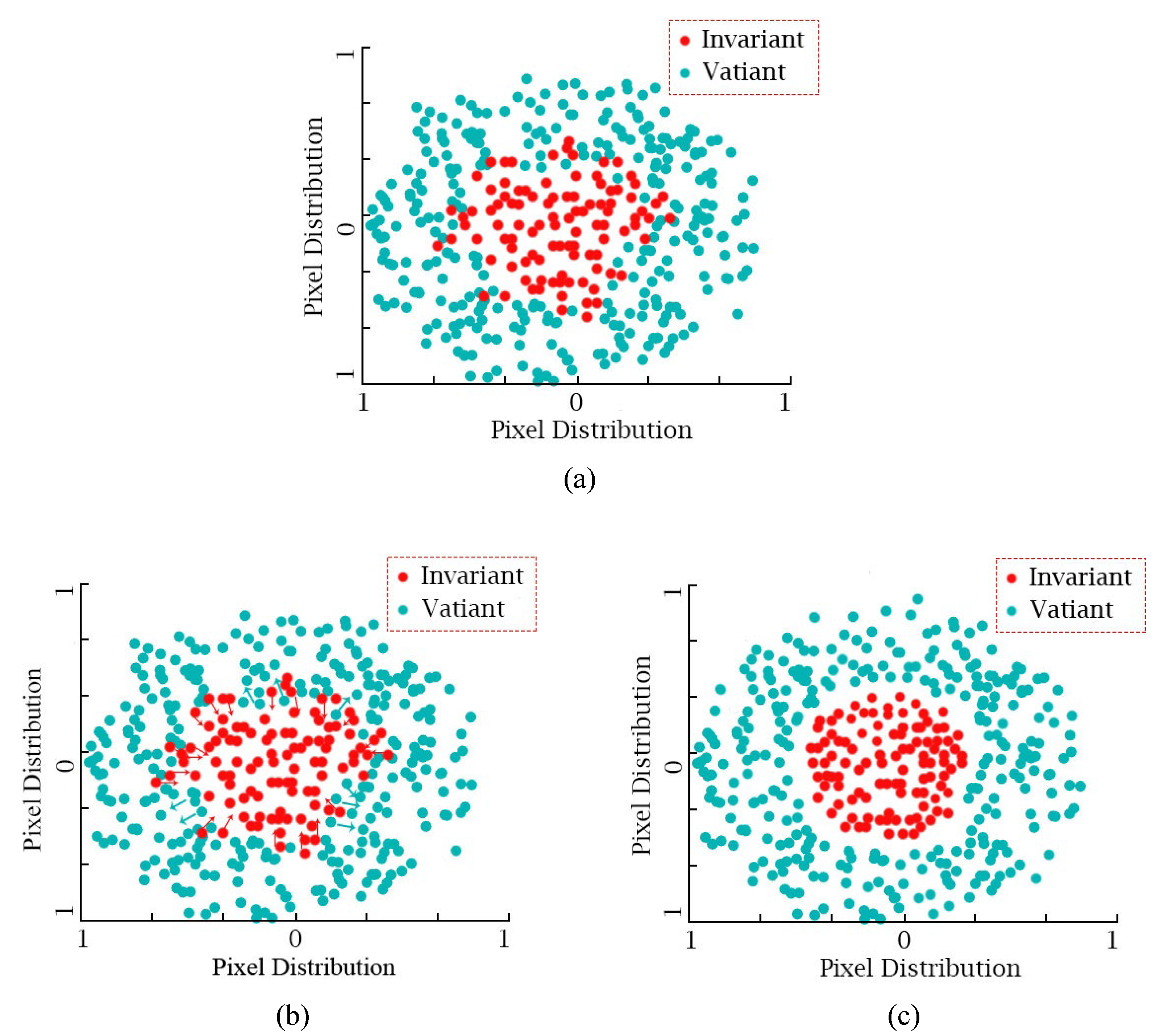
The USFA assigns two specific vector matrices to the bi-temporal projection features to suppress the invariant pixels and highlight the variant pixels. Figure 3 shows the visualization states of the invariant and variant pixels before/under/after the USFA algorithm, where the red dots represent the invariant pixels while the blue dots represent the variant pixels. Figure 3a shows the initial state of pixel features projected by Deep DNNs before USFA processing. It can be seen that some red dots and blue dots are on the edge of the threshold or in the opposite categories, which will lead to error classification of argument pixels. In Figure 3b, arrows near the intersection region of the red dots and blue dots represent their respective movement directions. It should be noted that not all feature distributions are suitable for the use of USFA. USFA plays a differential role for high-quality features to be processed. Therefore, in the case of erroneously dividing the invariant and variant features into the opposite categories, it will result in the amplification of error suppressing and highlighting. Figure 3c shows the redistribution of pixels after USFA processing, and it is easier to distinguish the invariant pixels from the variant pixels.
IRMAD is a widely used multivariate image alteration detection method. Its capability is to capture the multivariate alterations of unstable pixels on the premise of eliminating external interference factors. Through the linear transformation, the bi-temporal multivariate images, X and Y, captured over time can be expressed by coefficients, as shown in Equation (11).
where i denotes the number of spectral bands. We use to reflect the alterations of bi-temporal images. Once the maximum alteration intensity of the reference image and query image is obtained with small error by calculating the maximum variance of as shown in Equation (12), the problem will be solved. According to the CCA algorithm [35], to get the maximum , we just need to maximize Equation (12) according to constraint (13), where V denotes the mathematical variance.
In this way, the problem of bi-temporal multivariate image alteration detection is transformed into the problem of canonical correlation coefficient (CCC) . The larger CCC will lead to smaller value of Equation (12), which means a smaller alteration; on the contrary, smaller CCC means a greater alteration. On the other hand, the coefficients and will be obtained by CCA algorithm. Then, the alteration intensity of the bi-temporal images can be obtained by iteration of Chi-square distance, as shown in Equation (14). The iterative weight as shown in Equation (15), participates in the next variance of [11]. Iteration is repeated until the CCC converges, where and denote the number of iterations and the number of bands, respectively.
PCA is a lossy feature compression approach in essence. However, it is necessary to maintain the most original information in the compression process. To achieve this goal, the projection features should be scattered as much as possible. The scatter degree can be mathematically expressed by variance.
Suppose A is a feature after projection. The variance of A as shown in Equation (16) should be as large as possible to achieve the purpose of scattered projection features. Before PCA dimensionality reduction, Zero-mean has generally been done. For the convenience of calculation, Equation (16) can also be approximately expressed as Equation (17).
where , , , , represent the mathematical variance, band index, the number of bands, a value of feature A, and the mean value of feature A, respectively.
On the other side, in order to reduce the redundant information of features, we hope that the projection features have no relevance to each other; thus, covariance is employed to measure the feature irrelevance. Suppose A and B, expressed as Equation (18), are the two features after PCA dimensionality reduction. Then, the covariance of A and B can be expressed as Equation (19); we want it to be 0 to achieve irrelevance.
We then use Equation (18) to construct the covariance matrix and multiply it with , thus obtaining Equation (20).
It can be seen that the diagonal element of Equation (20) is the variance of A and B. With Equation (19) to be 0, then Equation (20) can be expressed as Equation (21).
Therefore, to achieve the purpose, the reduced data covariance matrix should meet the condition of diagonal matrix. Suppose that the original data, are dimensionally reduced by PCA to obtain data , which satisfies the Equation (22).
Suppose that and are the covariance of and . Then,
Therefore, it is only necessary to obtain P and make , which satisfies the condition of a diagonal matrix. Since is a Real Symmetric Matrix, we just need to diagonalize it. Thus far, the PCA problem is solved.
2.4. Chi-Square Distance and Thresholding
By passing the bi-temporal images’ data, and through the D-PRNs’ learning framework, the input images will be transformed into other new data spaces, denoted by and . As we know, projection features of a DNN with good construction can more accurately express the essence of the original images. However, it is difficult for us to judge whether a pixel has changed or not from the bi-temporal projection features. Therefore, an Alteration Intensity Map is used to comprehensively reflect the alteration degree of each pixel pairs of bi-temporal images. We used D, as Equation (24) shows, to represent the divergence of bi-temporal features and ; and it serves as the the principal component of Chi-square distance, as shown in Equation (25), which is employed to measure the alteration intensity of bi-temporal features
where denotes the transposition of vector matrix , while denotes the variance of the i-th band pair. The result of Chi-Square Distance is a data matrix for storing grayscale values. It represents the alteration degree of all pixel pairs.
The generated Alteration Intensity Map consists of gray scale values in the range of 0~255, which makes it difficult to judge whether or not any alteration happens. Therefore, a Binary Alteration Map is urgently necessary to indicate the altered pixels; thus, two threshold algorithms, K-means and Otsu, are respectively employed.
3. Experiments
In this section, two datasets, ‘River’ and ‘Taizhou’, were used for evaluating the performance of the proposed ADM-D-PRNs. Among them, ‘River’ is an opened hyperspectral dataset captured by a Hyperion sensor carried on satellite Earth Observing-1 (EO-1), while ‘Taizhou’ is a multispectral dataset captured by Landsat 7 Enhanced Thematic Mapper Plus (ETM+) sensor.
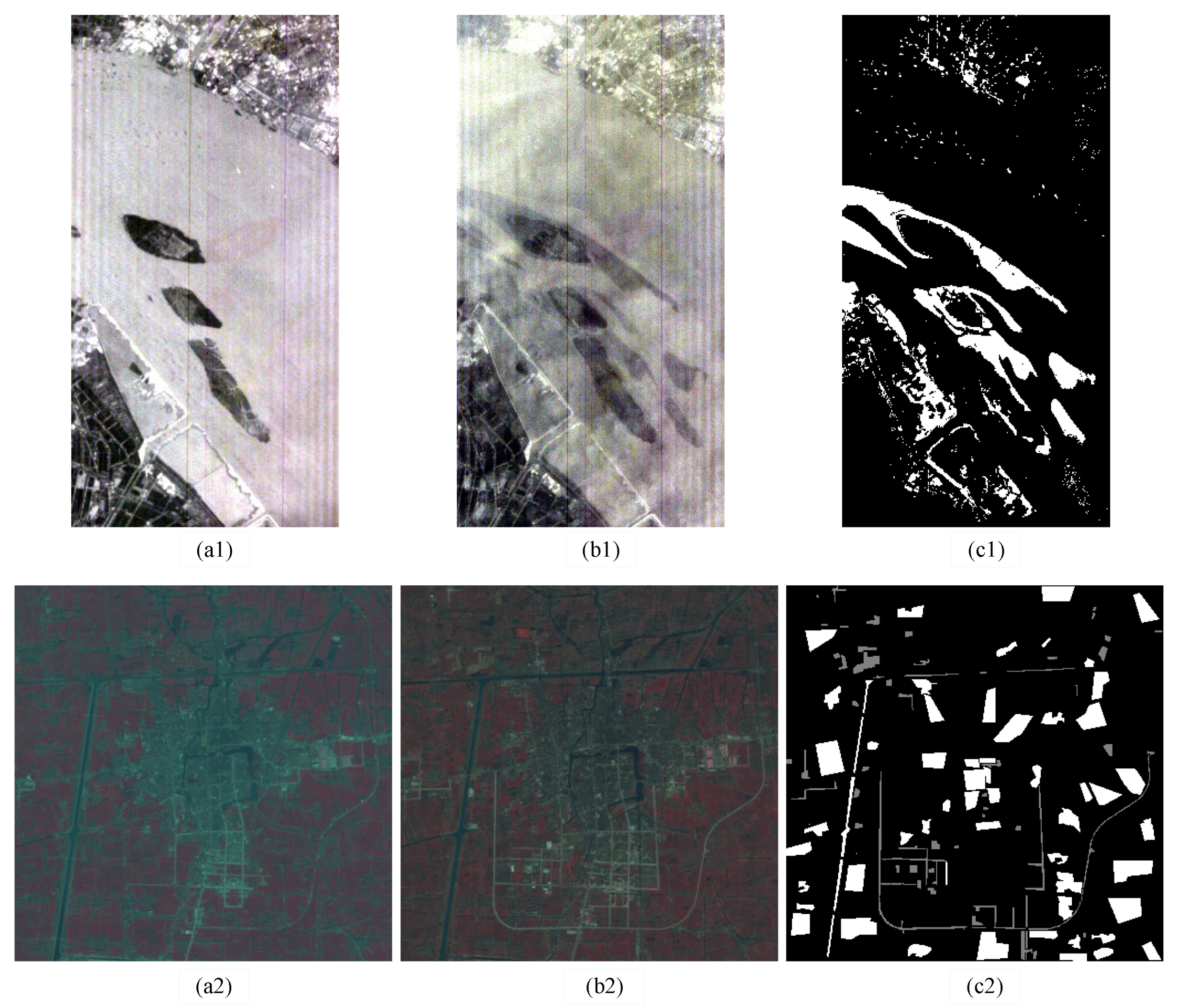
Figure 4 shows the tested datasets. Figure 4(a1,b1) represents the bi-temporal scene images of dataset ‘River’, captured on 3 May 2013 and 31 December 2013, respectively, in Jiangsu Province, China, with (a1) as reference image and (b1) as query image. Both of the two original images had the size of 463 × 241 × 198. The three number respectively denote the width, the height, and the number of testing spectral bands with 30-m spatial resolution. In the ground truth map, as Figure 4(c1) shows, the entire image belonged to the known areas, which consisted of 111,583 pixels, including 12,560 variant pixels marked with white and 99,023 invariant pixels marked with black. The alterations of dataset ‘River’ are the appearance and disappearance of prominent substances in the river channel.
Similarly, (a2) and (b2) represent the two scene images of dataset ‘Taizhou’, captured in 2000 and 2003, respectively, in Taizhou City, China, with (a2) as reference image and (b2) as query image. Both of the two original images had the size of 400 × 400 × 6, which means that the width and height of each original image were both 400 pixels. It had six testing multispectral bands (1 ~ 5 and 7) with 30-m spatial resolution, a dropping thermal infrared band (6) with 60-m spatial resolution, and a panchromatic band (8) with a resolution of 15 m. In the ground truth map of dataset ‘Taizhou’, as Figure 4(c2) shows, there were 160,000 pixels in total, 21,390 of which belonged to the known areas, including 4227 variant pixels marked with gray and 17,163 invariant pixels marked with white.
To measure the performance of the proposed ADM-D-PRNs, the five quantitative coefficients, OA_CHG, OA_UN, OA [36], Kappa, and F1 [37], as defined in Equations (26)–(30), were calculated.
where OA_CHG and OA_UN are two relatively one-sided coefficients, while OA, Kappa, and F1 are comprehensive coefficients. The four variables, TP (True Positives), FN (False Negatives), TN (True Negatives), and FP (False Positives), respectively, denote the number of variant pixels with correct hit, the number of invariant pixels with false hit, the number of invariant pixels with correct hit, and the number of variant pixels with false hit. The two constants GP (Ground-truth Positives) and GN (Ground-truth Negatives), respectively, denote the number of variant pixels and invariant pixels in a specific ground truth map; both of them are easily computed.
Figure 5 shows the visual analysis of the four variables, TP, FP, TN, and FN. In Figure 5(a1,a2) are two random Binary Alteration Maps of ‘River’ and ‘Taizhou’, where (b1,b2) show the corresponding ground truth maps and (c1,c2) display the corresponding Hitting Status Maps, which are employed to visualize various kinds of detection results. In order to generate the Hitting Status Maps, pixels of the Binary Alteration Map were compared with the corresponding pixels of the ground truth map. For dataset ‘River’, the TP and TN pixels were marked with white and black, while the FP and FN pixels were marked with yellow and red, as Figure 5(c1) shows. For dataset ‘Taizhou’, the TP and TN pixels were marked with red and green, while the FP and FN pixels were marked with white and blue, as Figure 5(c2) shows.
To show the superiority of the proposed ADM-D-PRNs, we employed the USFA, IRMAD, and PCA, respectively, with the proposed D-PRNs and we implemented the baseline DSFA [31] series models on two datasets, ‘River’ and ‘Taizhou,’ as well, for fair comparison. The DSFA-64-2, DSFA-128-2, and DSFA-256-2 were conducted. In the following, Section 3.1 and Section 3.2, we present the visualization results in different processes to demonstrate how the proposed models and baseline methods work. The Projection Feature Maps, Divergence Maps, and Binary Alteration Maps of the state-of-the-art baseline models, DSFA-64-2, DSFA-128-2, and DSFA-256-2, and the proposed ADM-D-PRNs are shown.
3.1. Projection Feature Maps
DNNs have powerful capability to transform the original image data into a new feature space non-linearly for alteration detection tasks. Since the spectral band number of a RGB image is up to 3 while each group of projection features has 10 bands, in this experiment, we used the remote sensing image processing tool ENVI 5.3 to choose the three bands (the fourth, the third, and the second bands) in the feature space, which were endowed with red, green, and blue color independently to synthesize the pseudo color images. Due to the characteristics of nonlinear expression capability of DNNs, each group of features projected by the same DNN in different training processes will differentially express the essence of the original images; thus, the pseudo color images of the corresponding projection features were also different in visual performance.
Figure 6 and Figure 7 show the bi-temporal pseudo color images of projection features on datasets ‘River’ and ‘Taizhou’, respectively, where (a), (b), (c), (d), (e), and (f) represent feature maps of DSFA-64-2, DSFA-128-2, DSFA-256-2, proposed ADM-D-PRNs using USFA, proposed ADM-D-PRNs using IRMAD, and proposed ADM-D-PRNs using PCA, respectively.
3.2. Detected Binary Alteration Maps
The arithmetic divergence between two feature sets is defined as Divergence Features. Similarly, for the generation of projection feature maps, shown in Figure 6 and Figure 7, we chose the same bands to synthesize the Divergence Maps. In Figure 8 and Figure 9, the first row (R1) shows the pseudo color Divergence Maps of datasets ‘River’ and ‘Taizhou’, respectively. It should be noted that, even if the different learning frameworks with infinite convergence obtained in different training processes had equivalent degrees of fitting, there were individual differences between the corresponding parameters of the two learning frameworks. It was a result of non-uniqueness of the Divergence Features.
Then, the second row (R2) shows the corresponding Alteration Intensity Maps. The alterations of bi-temporal images can be roughly reflected on the Alteration Intensity Map. The brightness of pixels in the Alteration Intensity Maps are defined according to the alteration probability being detected. In Figure 8(R2) and Figure 9(R2), the very bright areas indicate significant alteration, while the very dark areas indicate little or no alteration. It is worth noting that the accuracy of alteration intensity cannot be reflected by a single category of pixels, just as the highlighted component of the Alteration Intensity Map obtained by ADM-D-PRNs using IRMAD is much brighter than that using USFA. However, after the threshold segmentation, the detection performance of the former exceeded that of the latter. In view of this phenomenon, our explanation is that in the process of feature transformation, the highlighting of variant pixel features led to false highlighting of some invariant pixel features, and vice versa.
Finally, to show the results of the alteration detection task, we employed the K-means and Otsu as threshold algorithms to transform the Alteration Intensity Map into a binary representation that can uniquely determine whether pixels were altered or not. In Figure 8(R3) and Figure 9(R3,R4), the black and white pixels indicate the areas detected as invariant and variant, respectively. It should be noted that, in Figure 9(R3), the results indicated in white represent the variant area for the entire image, while those in Figure 9(R4) represent the variant area for the known areas. Since the unknown areas were not indicated in the ground truth map, they were not involved in the calculation of quantitative coefficients.
3.3. Comparison Results of Alteration Detection Results
In the following, Table 1, Table 2, Table 3 and Table 4, we give the quantitative results of alteration detection with the proposed ADM-D-PRNs and the state-of-the-art models DSFA-64-2, DSFA-128-2, and DSFA-256-2 proposed in [31]. The three post-processing methods, USFA, IRMAD, and PCA, were employed to evaluate and make up for the deficiency of the proposed D-PRNs. The threshold algorithms, K-means and Otsu methods, were respectively applied, and the comparison results are shown in Table 1, Table 2, Table 3 and Table 4. The figures demonstrate that the overall performance of the proposed ADM-D-PRNs was superior to the state-of-the-art DSFA series models.
Table 1 and 2 show the alteration detection results of dataset ‘River’ using K-means and Otsu, respectively. It can be seen from Table 1 that the proposed D-PRNs with USFA achieved the best OA and had a slight increase compared with the baseline method DSFA-128-2, while the proposed D-PRNs with PCA performed the best in one-sided coefficient, OA_CHG, with about a 6% rise and about 1.4% and 1.23% rises in comprehensive coefficients Kappa and F1, respectively, comparing with the best baseline model, DSFA-128-2. In Table 2, the comparison results indicated that the state-of-the-art DSFA series models did not own any top performance among the five quantitative coefficients. The best performances of both one-sided coefficient OA_UN and comprehensive coefficient OA were in the proposed model ADM-D-PRNs using USFA, while the proposed ADM-D-PRNs using PCA performed the best in one-sided coefficient OA_CHG and the other two comprehensive coefficients, Kappa and F1.
Similarly, Table 3 and Table 4 show the alteration detection results of dataset ‘Taizhou’ using K-means and Otsu, respectively. In Table 3, comparison results indicate that the proposed model sacrificed little performance in OA_UN coefficient and had great improvement in OA_CHG. The baseline method, DSFA-128-2, occupied the optimal value in OA_UN coefficient, while the proposed D-PRNs with PCA achieved the best performance in one-sided coefficient OA_CHG and comprehensive coefficients, Kappa and F1. In Table 4, the proposed D-PRNs with PCA performed the best in one-sided coefficient OA_CHG and all three comprehensive coefficients, OA, Kappa, and F1.
4. Discussion
In addition to the difference in the learning capability of Deep Networks, the number of samples and difference among individuals will affect the good construction of model parameters. Furthermore, in order to compare and analyze the difference in detection accuracy caused by various sampling strategies, we performed the proposed ADM-D-PRNs using USFA with five sampling strategies on datasets ‘River’ and ‘Taizhou’. As shown in Table 5 and Table 6, the Random, CVA_CHG, CVA_UN, G_CHG, and G_UN are five simple sampling strategies based on CVA pre-detection and ground truth map, and they, respectively, indicated random selection, variant pixel pairs corresponding to the CVA Binary Alteration Map, invariant pixel pairs corresponding to the CVA Binary Alteration Map, variant pixel pairs corresponding to the ground truth map, and invariant pixel pairs corresponding to the ground truth map. As the involved areas of the aforementioned sampling strategies provided enough pixel pairs as training samples, we did not need to consider the problem of generalization ability of the learning framework brought by insufficient samples.
In our experiments, we used a comprehensive F1 score to analyze the desirability and feasibility of several sampling strategies on two datasets as follows. First, the proposed ADM-D-PRNs with random strategy only achieved 0.7053 in F1 coefficient on dataset ‘River’. It is a large gap compared with the top two scores by conducting the CVA_UN and G_UN strategies. Moreover, once the random strategy is adopted in a learning process, the pre-detection will become meaningless. Second, similarly, CVA_CHG and G_CHG strategies contributed to high scores of 0.9581 and 0.9690 in F1, respectively, on the dataset ‘Taizhou’, but performed very poorly on dataset ‘River’. Our explanation for the anomaly is partly and chiefly that the altered pixels with less cardinality contained many pseudo changing features brought by hyperspectral imaging conditions, which greatly misled the deep learning. However, the problem was avoided when using CVA_CHG and G_CHG strategies on multispectral dataset ‘Taizhou’. This was mainly due to the multispectral dataset Taizhou containing fewer pseudo features. Third, CVA_UN and G_ UN achieved the top two values, of 0.7612 and 0.7608, in F1 coefficient on dataset ‘River’ and a very high accuracy, of 0.9541 and 0.9553, in the same coefficient on dataset ‘Taizhou’. However, since the ground truth map is used to verify the performance of alteration detection algorithms, G_UN should not be used in practical application. According to the above analysis, we adopted CVA_UN as a sampling strategy in the tests.
5. Conclusions
In this paper, we proposed the alteration detection model ADM-D-PRNs to detect the alterations of bi-temporal multispectral/hyperspectral remote sensing images. In the proposed ADM-D-PRNs’ schema, D-PRNs are used to transform the original bi-temporal images into a new dimensional space. We established USFA, IRMAD, and PCA as post-processing methods of projection features to evaluate and compensate the deficiency of deep networks. Our proposed D-PRNs are lightweight networks with unsupervised architecture; they can save a lot of learning time and do not need any absolutely trusted labels to guide the learning direction. We implemented the proposed schema on a hyperspectral dataset, ‘River’, and a multispectral dataset, ‘Taizhou’. Experimental results showed that the proposed model ADM-D-PRNs outperformed the state-of-the-art models DSFA-64-2, DSFA-128-2, and DSFA-256-2. This means the proposed D-PRNs have a more powerful capability to nonlinearly express the essential divergence of bi-temporal multispectral/hyperspectral images than the fully connected networks used in baselined DSFA series models.
Our proposed scheme adopted the CVA pre-detection method to generate the invariant pixel pairs as training samples, as mentioned in the Discussion. However, the premise of this sampling method is that sufficient invariant pixel pairs are needed. Otherwise, the expected purpose will not be achieved. Therefore, the future work is to formulate a robust sampling algorithm to quantify the importance of features and generate the suitable pixel pairs as training samples. In this way, we can get rid of the uncontrollable and unexpected results brought by the various pre-detection methods.
Author Contributions
Conceptualization, J.L., X.Y. and L.F.; Data curation, J.L.; Formal analysis, J.L.; Methodology, J.L. and X.Y.; Project administration, X.Y. and L.F.; Supervision, X.Y. and L.F.; Validation, J.L., X.Y. and L.F.; Visualization, J.L.; Writing–original draft, J.L.; Writing–review and editing, X.Y. All authors have read and agreed to the published version of the manuscript.
Funding
This research was funded by the National Natural Science Foundation of China, grant number 61902448.
Institutional Review Board Statement
Not applicable.
Informed Consent Statement
Not applicable.
Data Availability Statement
Not applicable.
Acknowledgments
We thank Hailun Liang for valuable discussion and assistance with problems encountered in the experiment. In particular, he provided an effective solution for the incapability of deep learning on dataset ‘Hermiston’.
Conflicts of Interest
The authors declare that there is no conflict of interest regarding the publication of this paper.
References
- Zhou, H.; Liu, S.; He, J.; Wen, Q.; Song, L.; Ma, Y. A new model for the automatic relative radiometric normalization of multiple images with pseudo-invariant features. Int. J. Remote. Sens. 2016, 37, 4554–4573. [Google Scholar] [CrossRef]
- Schott, J.R.; Salvaggio, C.; Volchok, W.J. Radiometric scene normalization using pseudoinvariant features. Remote Sens. Environ. 1988, 26, 1–16. [Google Scholar] [CrossRef]
- Cheng, X.-Y.; Zhuang, X.-Q.; Zhang, D.; Yao, Y.; Hou, J.; He, D.-G.; Jia, J.-X.; Wang, Y.-M. A relative radiometric correction method for airborne SWIR hyperspectral image using the side-slither technique. Opt. Quantum Electron. 2019, 51, 105. [Google Scholar] [CrossRef]
- Li, Z.; Shen, H.; Cheng, Q.; Li, W.; Zhang, L. Thick Cloud Removal in High-Resolution Satellite Images Using Stepwise Radiometric Adjustment and Residual Correction. Remote Sens. 2019, 11, 1925. [Google Scholar] [CrossRef] [Green Version]
- Cao, P.; Zhang, S. Research on image recognition of Wushu action based on remote sensing image and embedded system. Microprocess. Microsyst. 2021, 82, 103841. [Google Scholar] [CrossRef]
- Zyurt, F. Efficient deep feature selection for remote sensing image recognition with fused deep learning architectures. J. Supercomput. 2020, 76, 1–19. [Google Scholar] [CrossRef]
- You, H.; Tian, S.; Yu, L.; Lv, Y. Pixel-Level Remote Sensing Image Recognition Based on Bidirectional Word Vectors. IEEE Trans. Geosci. Remote Sens. 2019, 58, 1281–1293. [Google Scholar] [CrossRef]
- Chebbi, I.; Mellouli, N.; Farah, I.; Lamolle, M. Big Remote Sensing Image Classification Based on Deep Learning Extraction Features and Distributed Spark Frameworks. Big Data Cogn. Comput. 2021, 5, 21. [Google Scholar] [CrossRef]
- Alhassan, V.; Henry, C.; Ramanna, S.; Storie, C. A deep learning framework for land-use/land-cover mapping and analysis using multispectral satellite imagery. Neural Comput. Appl. 2019, 32, 8529–8544. [Google Scholar] [CrossRef]
- Nielsen, A.A.; Conradsen, K.; Simpson, J.J. Multivariate alteration detection (MAD) and MAF postprocessing in multispectral, bitemporal image data: New approaches to change detection studies. Remote Sens. Environ. 1998, 64, 1–19. [Google Scholar] [CrossRef] [Green Version]
- Nielsen, A.A. The Regularized Iteratively Reweighted MAD Method for Change Detection in Multi- and Hyperspectral Data. IEEE Trans. Image Process. 2007, 16, 463–478. [Google Scholar] [CrossRef] [PubMed] [Green Version]
- Wold, S.; Esbensen, K.; Geladi, P. Principal component analysis. Chemom. Intell. Lab. Syst. 1987, 2, 37–52. [Google Scholar] [CrossRef]
- Marchesi, S.; Bruzzone, L. Ica and Kernel Ica for Change Detection in Multispectral Remote Sensing Images, 2009 IEEE International Geoscience and Remote Sensing Symposium, Cape Town, South Africa. IEEE 2009, 2, 980–983. [Google Scholar] [CrossRef]
- Collins, J.B.; Woodcock, C.E. Change detection using the Gramm-Schmidt transformation applied to mapping forest mortality. Remote Sens. Environ. 1994, 50, 267–279. [Google Scholar] [CrossRef]
- Wei, Y.; Liu, H.; Song, W.; Yu, B.; Xiu, C. Normalization of time series DMSP-OLS nighttime light images for urban growth analysis with Pseudo Invariant Features. Landsc. Urban. Plan. 2014, 128, 1–13. [Google Scholar] [CrossRef]
- Zhan, Y.; Fu, K.; Yan, M.; Sun, X.; Wang, H.; Qiu, X. Change Detection Based on Deep Siamese Convolutional Network for Optical Aerial Images. IEEE Geosci. Remote Sens. Lett. 2017, 14, 1845–1849. [Google Scholar] [CrossRef]
- Gong, M.; Zhao, J.; Liu, J.; Miao, Q.; Jiao, L. Change Detection in Synthetic Aperture Radar Images Based on Deep Neural Networks. IEEE Trans. Neural Netw. Learn. Syst. 2015, 27, 125–138. [Google Scholar] [CrossRef] [PubMed]
- Liu, J.; Gong, M.; Qin, K.; Zhang, P. A Deep Convolutional Coupling Network for Change Detection Based on Heterogeneous Optical and Radar Images. IEEE Trans. Neural Netw. Learn. Syst. 2016, 29, 545–559. [Google Scholar] [CrossRef]
- Zhang, C.; Yue, P.; Tapete, D.; Jiang, L.; Shangguan, B.; Huang, L.; Liu, G. A deeply supervised image fusion network for change detection in high resolution bi-temporal remote sensing images. ISPRS J. Photogramm. Remote Sens. 2020, 166, 183–200. [Google Scholar] [CrossRef]
- Zhao, W.; Wang, Z.; Gong, M.; Liu, J. Discriminative Feature Learning for Unsupervised Change Detection in Heterogeneous Images Based on a Coupled Neural Network. IEEE Trans. Geosci. Remote Sens. 2017, 55, 7066–7080. [Google Scholar] [CrossRef]
- Zhang, M.; Shi, W. A Feature Difference Convolutional Neural Network-Based Change Detection Method. IEEE Trans. Geosci. Remote Sens. 2020, 58, 7232–7246. [Google Scholar] [CrossRef]
- Liu, F.; Jiao, L.; Tang, X.; Yang, S.; Ma, W.; Hou, B. Local Restricted Convolutional Neural Network for Change Detection in Polarimetric SAR Images. IEEE Trans. Neural Netw. Learn. Syst. 2019, 30, 818–833. [Google Scholar] [CrossRef]
- Liu, X.; Lathrop, R., Jr. Urban change detection based on an artificial neural network. Int. J. Remote Sens. 2002, 23, 2513–2518. [Google Scholar] [CrossRef]
- Georgakopoulos, S.V.; Tasoulis, S.K.; Mallis, G.I.; Vrahatis, A.G.; Plagianakos, V.P.; Maglogiannis, I.G. Change detection and convolution neural networks for fall recognition. Neural Comput. Appl. 2020, 32, 17245–17258. [Google Scholar] [CrossRef]
- Ghosh, S.; Roy, M.; Ghosh, A. Semi-supervised change detection using modified self-organizing feature map neural network. Appl. Soft Comput. 2014, 15, 1–20. [Google Scholar] [CrossRef]
- Connors, C.; Vatsavai, R.R. Semi-Supervised Deep Generative Models for Change Detection in Very High Resolution Imagery. In Proceedings of the 2017 IEEE International Geoscience and Remote Sensing Symposium, Fort Worth, TX, USA, IEEE. 23–28 July 2017; pp. 1063–1066. [Google Scholar] [CrossRef]
- Chen, H.; Wu, C.; Du, B.; Zhang, L.; Wang, L. Change Detection in Multisource VHR Images via Deep Siamese Convolutional Multiple-Layers Recurrent Neural Network. IEEE Trans. Geosci. Remote Sens. 2019, 58, 2848–2864. [Google Scholar] [CrossRef]
- Andermatt, P.; Timofte, R. A Weakly Supervised Convolutional Network for Change Segmentation and Classification; Springer: Cham, Switzerland, 2021; Volume 12628, pp. 103–119. [Google Scholar] [CrossRef]
- Daudt, R.C.; Le Saux, B.; Boulch, A.; Gousseau, Y. Weakly supervised change detection using guided anisotropic diffusion. Mach. Learn. 2021, 1–27. [Google Scholar] [CrossRef]
- Zhang, M.; Xu, G.; Chen, K.; Yan, M.; Sun, X. Triplet-Based Semantic Relation Learning for Aerial Remote Sensing Image Change Detection. IEEE Geosci. Remote Sens. Lett. 2018, 16, 266–270. [Google Scholar] [CrossRef]
- Du, B.; Ru, L.; Wu, C.; Zhang, L. Unsupervised Deep Slow Feature Analysis for Change Detection in Multi-Temporal Remote Sensing Images. IEEE Trans. Geosci. Remote Sens. 2019, 57, 9976–9992. [Google Scholar] [CrossRef] [Green Version]
- Kanungo, T.; Mount, D.M.; Netanyahu, N.S.; Piatko, C.D.; Silverman, R.; Wu, A.Y. An efficient k-means clustering algorithm: Analysis and implementation. IEEE Trans. Pattern Anal. Mach. Intell. 2002, 24, 881–892. [Google Scholar] [CrossRef]
- Otsu, N. A Threshold Selection Method from Gray-Level Histograms. IEEE Trans. Syst. Man Cybern. 1979, 9, 62–66. [Google Scholar] [CrossRef] [Green Version]
- Danielsson, P.-E. Euclidean Distance Mapping. Comput. Graph. Image Process. 1980, 14, 227–248. [Google Scholar] [CrossRef] [Green Version]
- Hardoon, D.R.; Szedmak, S.; Shawe-Taylor, J. Canonical correlation analysis: An overview with application to learning methods. Neural Comput. 2004, 16, 2639–2664. [Google Scholar] [CrossRef] [PubMed] [Green Version]
- Wang, D.; Gao, T.; Zhang, Y. Image Sharpening Detection Based on Difference Sets. IEEE Access 2020, 8, 51431–51445. [Google Scholar] [CrossRef]
- De Bem, P.P.; de Carvalho Junior, O.A.; Guimarães, R.F.; Gomes, R.A.T. Change Detection of Deforestation in the Brazilian Amazon Using Landsat Data and Convolutional Neural Networks. Remote Sens. 2020, 12, 901. [Google Scholar] [CrossRef] [Green Version]
Figure 1.
The proposed ADM-D-PRNs.

Figure 2.
Structure of proposed Dual-path Partial Recurrent Networks (D-PRNs).

Figure 3.
Alterations in pixel distribution: (a) before USFA, (b) under USFA, and (c) after USFA.

Figure 4.
Tested datasets ‘River’ and ‘Taizhou’; (a1,b1): scene images of dataset ‘River’; (c1): the ground truth map of dataset ‘River’; (a2,b2): scene images of dataset ‘Taizhou’; (c2): the ground truth map of dataset ‘Taizhou’.
Figure 4.
Tested datasets ‘River’ and ‘Taizhou’; (a1,b1): scene images of dataset ‘River’; (c1): the ground truth map of dataset ‘River’; (a2,b2): scene images of dataset ‘Taizhou’; (c2): the ground truth map of dataset ‘Taizhou’.

Figure 5.
Visualization of Hitting Status Maps; (a1,a2): the two random Binary Alteration Map of datasets ‘River’ and ‘Taizhou’; (b1,b2): the corresponding ground truth maps; (c1,c2): the corresponding Hitting Status Maps.
Figure 5.
Visualization of Hitting Status Maps; (a1,a2): the two random Binary Alteration Map of datasets ‘River’ and ‘Taizhou’; (b1,b2): the corresponding ground truth maps; (c1,c2): the corresponding Hitting Status Maps.

Figure 6.
Bi-temporal pseudo color images of projection features by performing: (a) DSFA-64-2, (b) DSFA-128-2, (c) DSFA-256-2, (d) ADM-D-PRNs using USFA, (e) ADM-D-PRNs using IRMAD, and (f) ADM-D-PRNs using PCA, on dataset ‘River’.
Figure 6.
Bi-temporal pseudo color images of projection features by performing: (a) DSFA-64-2, (b) DSFA-128-2, (c) DSFA-256-2, (d) ADM-D-PRNs using USFA, (e) ADM-D-PRNs using IRMAD, and (f) ADM-D-PRNs using PCA, on dataset ‘River’.

Figure 7.
Bi-temporal pseudo color images of projection features by performing: (a) DSFA-64-2, (b) DSFA-128-2, (c) DSFA-256-2, (d) ADM-D-PRNs using USFA, (e) ADM-D-PRNs using IRMAD, and (f) ADM-D-PRNs using PCA, on dataset ‘Taizhou’.
Figure 7.
Bi-temporal pseudo color images of projection features by performing: (a) DSFA-64-2, (b) DSFA-128-2, (c) DSFA-256-2, (d) ADM-D-PRNs using USFA, (e) ADM-D-PRNs using IRMAD, and (f) ADM-D-PRNs using PCA, on dataset ‘Taizhou’.

Figure 8.
Visualization results of different operation stages on dataset ‘River’; (R1) Divergence Maps, (R2) Alteration Intensity Maps, and (R3) Binary Alteration Maps; (C1) DSFA-64-2, (C2) DSFA-128-2, (C3) DSFA-256-2, (C4) ADM-D-PRNs using USFA, (C5) ADM-D-PRNs using IRMAD, and (C6) ADM-D-PRNs using PCA.

Figure 9.
Visualization results of different operation stages on dataset ‘Taizhou’; (R1) Divergence Maps, (R2) Alteration Intensity Maps, (R3) Binary Alteration Maps (entire image), and (R4) Binary Alteration Maps (known areas); (C1) DSFA-64-2, (C2) DSFA-128-2, (C3) DSFA-256-2, (C4) ADM-D-PRNs using USFA, (C5) ADM-D-PRNs using IRMAD, and (C6) ADM-D-PRNs using PCA.


Table 1.
Alteration detection results of dataset ‘River’ using K-means.
| Methods | DSFA-64-2 [31] | DSFA-128-2 [31] | DSFA-256-2 [31] | ADM-D-PRNs Using USFA (Proposed) | ADM-D-PRNs Using IRMAD (Proposed) | ADM-D-PRNs Using PCA (Proposed) |
|---|---|---|---|---|---|---|
| GP GN | 12,560 | |||||
| 99,023 | ||||||
| TP TN | 7707 | 8478 | 8319 | 8911 | 9235 | 9248 |
| 97,162 | 97,149 | 96,463 | 97,109 | 96,398 | 96,607 | |
| FP FN | 1861 | 1874 | 2560 | 1914 | 2625 | 2416 |
| 4853 | 4082 | 4241 | 3649 | 3325 | 3312 | |
| OA_CHG OA_UN | 0.6136 | 0.6750 | 0.6623 | 0.7095 | 0.7353 | 0.7363 |
| 0.9812 | 0.9811 | 0.9741 | 0.9807 | 0.9735 | 0.9756 | |
| OA Kappa | 0.9398 | 0.9466 | 0.9390 | 0.9501 | 0.9467 | 0.9487 |
| 0.6639 | 0.7106 | 0.6760 | 0.7344 | 0.7264 | 0.7348 | |
| F1 | 0.6966 | 0.7400 | 0.7098 | 0.7621 | 0.7563 | 0.7635 |
Table 2.
Alteration detection results of dataset ‘River’ using Otsu.
| Methods | DSFA-64-2 [31] | DSFA-128-2 [31] | DSFA-256-2 [31] | ADM-D-PRNs Using USFA (Proposed) | ADM-D-PRNs Using IRMAD (Proposed) | ADM-D-PRNs Using PCA (Proposed) |
|---|---|---|---|---|---|---|
| GP GN | 12,560 | |||||
| 99,023 | ||||||
| TP TN | 7667 | 8342 | 8298 | 8530 | 8970 | 9225 |
| 97,192 | 97,267 | 96,483 | 97,546 | 96,984 | 96,720 | |
| FP FN | 1831 | 1756 | 2540 | 1477 | 2039 | 2303 |
| 4893 | 4218 | 4262 | 4030 | 3590 | 3335 | |
| OA_CHG OA_UN | 0.6104 | 0.6642 | 0.6623 | 0.6791 | 0.7142 | 0.7345 |
| 0.9815 | 0.9823 | 0.9741 | 0.9851 | 0.9794 | 0.9767 | |
| OA Kappa | 0.9397 | 0.9465 | 0.9390 | 0.9506 | 0.9496 | 0.9495 |
| 0.6624 | 0.7069 | 0.7284 | 0.7289 | 0.7331 | 0.7377 | |
| F1 | 0.6952 | 0.7363 | 0.7098 | 0.7560 | 0.7612 | 0.7659 |
Table 3.
Alteration detection results of dataset ‘Taizhou’ using K-means.
| Methods | DSFA-64-2 [31] | DSFA-128-2 [31] | DSFA-256-2 [31] | ADM-D-PRNs Using USFA (Proposed) | ADM-D-PRNs Using IRMAD (Proposed) | ADM-D-PRNs Using PCA (Proposed) |
|---|---|---|---|---|---|---|
| GP GN | 4227 | |||||
| 17,163 | ||||||
| TP TN | 3673 | 3769 | 3538 | 3942 | 4061 | 4112 |
| 16,954 | 17,104 | 17,117 | 17,069 | 16,900 | 16,898 | |
| FP FN | 209 | 59 | 46 | 94 | 263 | 265 |
| 554 | 458 | 689 | 285 | 166 | 115 | |
| OA_CHG OA_UN | 0.8689 | 0.8916 | 0.8370 | 0.9326 | 0.9607 | 0.9728 |
| 0.9878 | 0.9966 | 0.9973 | 0.9945 | 0.9847 | 0.9846 | |
| OA Kappa | 0.9643 | 0.9758 | 0.9656 | 0.9823 | 0.9799 | 0.9822 |
| 0.8839 | 0.9210 | 0.8851 | 0.9432 | 0.9373 | 0.9447 | |
| F1 | 0.9059 | 0.9358 | 0.9059 | 0.9541 | 0.9493 | 0.9558 |
Table 4.
Alteration detection results of dataset ‘Taizhou’ using Otsu.
| Methods | DSFA-64-2 [31] | DSFA-128-2 [31] | DSFA-256-2 [31] | ADM-D-PRNs Using USFA (Proposed) | ADM-D-PRNs Using IRMAD (Proposed) | ADM-D-PRNs Using PCA (Proposed) |
|---|---|---|---|---|---|---|
| GP GN | 4227 | |||||
| 17,163 | ||||||
| TP TN | 3662 | 3759 | 3529 | 3955 | 4062 | 4119 |
| 16,958 | 17,112 | 17,120 | 17,065 | 16,893 | 16,892 | |
| FP FN | 205 | 51 | 43 | 87 | 270 | 271 |
| 565 | 468 | 698 | 295 | 165 | 108 | |
| OA_CHG OA_UN | 0.8663 | 0.8893 | 0.8349 | 0.9302 | 0.9610 | 0.9744 |
| 0.9881 | 0.9970 | 0.9975 | 0.9949 | 0.9843 | 0.9842 | |
| OA Kappa | 0.9640 | 0.9757 | 0.9654 | 0.9821 | 0.9797 | 0.9823 |
| 0.8827 | 0.9205 | 0.8840 | 0.9426 | 0.9365 | 0.9449 | |
| F1 | 0.9049 | 0.9354 | 0.9050 | 0.9537 | 0.9492 | 0.9560 |
Table 5.
Alteration detection results of dataset ‘River’ using different sampling strategies.
| Sampling | Random | CVA_CHG | CVA_UN | G_CHG | G_UN |
|---|---|---|---|---|---|
| OA_CHG OA_UN | 0.6323 | 0.3356 | 0.7088 | 0.9023 | 0.7072 |
| 0.9796 | 0.6947 | 0.9805 | 0.5512 | 0.9807 | |
| OA Kappa | 0.9405 | 0.6543 | 0.9499 | 0.5907 | 0.9499 |
| 0.6727 | 0.0172 | 0.7334 | 0.1812 | 0.7330 | |
| F1 | 0.7053 | 0.1794 | 0.7612 | 0.3317 | 0.7608 |
Table 6.
Alteration detection results of dataset ‘Taizhou’ using different sampling strategies.
| Sampling | Random | CVA_CHG | CVA_UN | G_CHG | G_UN |
|---|---|---|---|---|---|
| OA_CHG OA_UN | 0.9342 | 0.9470 | 0.9326 | 0.9562 | 0.9357 |
| 0.9948 | 0.9927 | 0.9945 | 0.9957 | 0.9943 | |
| OA Kappa | 0.9828 | 0.9836 | 0.9823 | 0.9879 | 0.9827 |
| 0.9448 | 0.9479 | 0.9432 | 0.9614 | 0.9446 | |
| F1 | 0.9555 | 0.9581 | 0.9541 | 0.9690 | 0.9553 |
Publisher’s Note: MDPI stays neutral with regard to jurisdictional claims in published maps and institutional affiliations. |
© 2021 by the authors. Licensee MDPI, Basel, Switzerland. This article is an open access article distributed under the terms and conditions of the Creative Commons Attribution (CC BY) license (https://creativecommons.org/licenses/by/4.0/).
Share and Cite
MDPI and ACS Style
Li, J.; Yuan, X.; Feng, L. Alteration Detection of Multispectral/Hyperspectral Images Using Dual-Path Partial Recurrent Networks. Remote Sens. 2021, 13, 4802. https://doi.org/10.3390/rs13234802
AMA Style
Li J, Yuan X, Feng L. Alteration Detection of Multispectral/Hyperspectral Images Using Dual-Path Partial Recurrent Networks. Remote Sensing. 2021; 13(23):4802. https://doi.org/10.3390/rs13234802
Chicago/Turabian StyleLi, Jinlong, Xiaochen Yuan, and Li Feng. 2021. "Alteration Detection of Multispectral/Hyperspectral Images Using Dual-Path Partial Recurrent Networks" Remote Sensing 13, no. 23: 4802. https://doi.org/10.3390/rs13234802
Note that from the first issue of 2016, this journal uses article numbers instead of page numbers. See further details here.