
Study on Gage Widening Methods for Small-Radius Curves


China Academy of Railway Sciences Corporation Limited, Beijing 100081, China
*
Authors to whom correspondence should be addressed.
Appl. Sci. 2021, 11(12), 5334; https://doi.org/10.3390/app11125334
Submission received: 26 April 2021
/
Revised: 3 June 2021
/
Accepted: 3 June 2021
/
Published: 8 June 2021
(This article belongs to the Section Civil Engineering)
Abstract
:Existing gage widening standards and the influence of gage widening on the curve passing performance of trains and rail wear were examined. The existing gage widening theory can determine the minimum curve radius that needs to be widened, the widening value required by curves with different radii, and whether multiaxle locomotives can pass small-radius curves. However, it does not quantify the influence of the gage widening value on the curve passing performance and track maintenance workload. The range of the minimum curve radius that needs to be widened is 220–350 m, whereas some countries adopt a radius of 600 m; the maximum gage widening range is 15–20 mm, and few countries adopt gage widening values exceeding 30 mm. When the gage widening value increases from 0 to 10 mm, the lateral force of the curved wheel or rail with a radius less than 300 m is reduced by 16–20%, and that with a radius exceeding 300 m is reduced by 10–15%. The results of this study reveal that using proper gage widening values can reduce the lateral force of the wheel or rail and improve the curve passing performance. In the rail lifecycle, the implementation of the current gage widening standard requires only one gage adjustment operation, whereas the implementation of the original gage widening standard requires doubling gage adjustment operations.
1. Introduction
Gage widening on small-radius curves is essential to ensure that the rolling stock passes the curve safely and smoothly and to reduce driving resistance, rail wear, and the dynamic effect of the rolling stock on the track. The gage widening value is closely related to the radius of the curve, the wheelbase of the rolling stock, and the clearance between the wheel flange and gage line [1,2,3,4]. The smaller the radius of the curve and the rail gap, the larger the required wheelbase and gage widening value. An insufficient gage widening value increases the dynamic effect of the rail, driving resistance, and rail wear, whereas an excessive gage widening value increases the rail gap and reduces train stability.
Scholars have developed two gage widening theories for determining the gage widening value―geometric inscribing and dynamic inscribing―based on the running posture of the bogie curve when passing through the curve [5,6,7]. Geometric inscribing is divided into free inscribing, forced inscribing, and wedge-shaped inscribing. Dynamic inscribing is derived from geometric inscribing and free inscribing. Based on the parameters of vehicles operated by railway operators in various countries, a specific gage widening theory is selected to formulate the gage widening standard in a given case.
In this paper, we analyzed the existing calculation methods of gage widening and summarized the standards and related research of gage widening in various countries. A theoretical simulation analysis model was established to analyze the impact of gage widening on vehicle curve passing performance and rail wear. The influence of gage widening on field maintenance workload was studied through field investigation. Based on the above work, this paper discusses the rationality of current gage widening standards in China, providing a reference for finding reasonable values for gage widening.
2. Gage Widening Calculation Methods
2.1. Geometrically Free Inscribing
Figure 1 shows the determination of the gage widening value according to geometrically free inscribing theory. It assumes that no relative angle exists between the bogie and car body when the bogie passes through the curve; i.e., the shaft trail is in the radial position, the steel rail on the curve is in contact with the wheel rim in the outer guide shaft, and the steel rail under the curve is in contact with the wheel rim on the inner shaft trail. A gage value that is precisely sufficient to make the wheel rim contact but does not produce guiding force is the critical value of the geometrically free-inscribed gage, which can be calculated using Equation (1).
Here, represents the critical value of the free-inscribed gage; represents the maximum wheel set width; represents the outer vector distance, with its value given as ; represents the fixed wheelbase of the bogie; and represents the radius of the curve.
Next, the curve gage widening value e corresponding to the radius can be calculated using Equation (2):
Here, represents the standard gage, and a negative value of implies that the gage does not require widening.
2.2. Dynamically Free Inscribing
Dynamic inscribing means that when the bogie passes through the curve, the guiding force between the wheel and rail changes with many factors, including speed, height, axle load, and wheelbase; in addition, the principle of the minimum guiding force is used to determine the geometric position of the bogie on the curve and further calculate the required gage widening value according to the geometric position.
As shown in Figure 2, mechanically free inscribing of the bogie means that when the bogie passes through a curve, only the rim of the outer wheel of the front axle and the inner surface of the rail experience a lateral guiding force , and no lateral force exists between the rim of the other wheels and the rail. The vertical load applied to the top surface of the rail by the front and rear axle wheel treads is (wheel weight). When the bogie rotates around the center of rotation , the rotational torque generated by the frictional force between the wheel tread and the top surface of the rail is and , respectively, and is the rotation radius of the front axle wheel tread contact point around the center of rotation . Furthermore, is the rotation radius of the rear axle wheel tread contact point around the center of rotation
The torque balance equation of the bogie around the center of rotation in the track surface is given by Equation (3):
Here, represents the distance from the instantaneous center of rotation to the front axle, and represents the lateral force acting on the bogie core, which can be calculated using Equations (4)–(6) as follows.
In the above equations, represents the maximum load of the bogie; represents the speed; represents the acceleration of gravity; represents the curve radius; represents the superelevation of the curve; and represents the distance between the contact points on the top surface of the rail.
According to the minimum guiding force , the value of at different curve radii, outer rail superelevations, and driving speeds is calculated according to Equations (3)–(6). After the value of is determined (see Equation (7)) according to the geometric relationship shown in Figure 3, the minimum value of the normal rail wheel flange and gage line, , which is necessary for calculating the outer wheels of the rear axle of the bogie based on mechanically free inscribing, the gage widening value can be calculated using Equation (8).
2.3. Geometric Wedge and Normal Forced Inscribing
Wedge-shaped inscribing is generally utilized for multiaxle bogies. Here, a four-axle bogie is used as an example to show the wedge-shaped inscribed state. The outer rails are in contact with the outer wheel rims of the two end axles, and the inner rails are in contact with the inner wheel rims of the intermediate axle, as shown in Figure 4. The gage that satisfies the wedge-shaped inscribed state can be calculated using Equation (9). Normal forced inscribing increases half of the minimum rail gap based on the wedge-shaped inscribed gage, which is expressed as Equation (10).
In Equations (9) and (10), represents the critical value of the wedge-shaped inscribed gage; represents the maximum wheel set width; represents the outer vector distance formed by the first and fourth axles of the bogie, and its value is given by ; represents the inner vector distance formed by the second and third axles of the bogie, and its value is given as ; represents the minimum wheel flange gap (the sum of the rail gaps on both sides); and represents the sum of the free transverse momentum of the externally and internally connected peg shafts (transverse gap of the axle box).
3. Status of Gage Widening Standards
Gage widening standards for small-radius curve sections in the Soviet Union, the United States, Japan, and Germany have been summarized below to analyze the applications of gage widening theories and standards.
In 1936, based on a bogie with a wheelbase of 3.9 m and a rail gap of 11 mm, the Soviet Union adopted geometrically free inscribing to determine the gage widening value. As listed in Table 1, the minimum radius to be widened was 650 m, and the maximum widening amount was 16 mm, divided into four levels.
In 1957, the Soviet Union adopted dynamically free inscribing to readjust the gage widening value. As listed in Table 2, the minimum radius to be widened was 350 m and the maximum widening amount was 16 mm, divided into three levels; this approach was formally implemented in 1961 [8,9,10].
As shown in Table 3, at present, the current standards of Russia have been slightly adjusted. When the radius is less than or equal to 299 m, the gage is widened by 15 mm. When the radius is between 300 and 349 m, the gage is widened by 10 mm, and when the radius is greater than or equal to 350 m, the gage is not widened.
In 1921, the gage widening amount for American railways was determined based on the normal forced inscribing conditions of the two-axle bogie, as listed in Table 4. The minimum radius to be widened was 219 m, the maximum widening amount was 15.6 mm, and the progressive amount was 3.12 mm. The widening amount was divided into six levels [11,12].
However, current US standards do not recommend gage widening on curves because of problems associated with hollow tread-worn wheels, poor curving performance, and high wheel–rail contact stresses, which generate fatigue defects. Instead of altering gages, some researchers use rail profile grinding to improve the interface between wheels and rails on curves.
Japanese railways use a three-axle bogie with a wheelbase of 4.6 m and a rail gap of 7 mm; the gage widening value therein is determined based on geometrically free inscribing. The centers of the second and third axles are in the radial position (Figure 5); Equation (11) was formulated to calculate gage widening values listed in Table 5. The minimum radius to be widened is 600 m, the maximum widening amount is 30 mm, and the progressive amount is 5 mm; the widening amount is divided into seven levels [13,14,15].
In 1958, the gage widening values for West German railways were calculated according to wedge-shaped inscribing, as shown in Equation (12) and listed in Table 6. The minimum radius to be widened was 200 m, the maximum widening amount was 20 mm, and the progressive amount was 5 mm, divided into five levels.
Here, represents the fixed distance of the bogie (m), represents the curve radius (m), represents the standard gap between the wheel and the rail (mm), represents the transverse momentum of the intermediate shaft (mm), represents the intermediate shaft flange wear (mm), and represents the squeezing amount of the track at the position of the intermediate shaft (mm).
During the operation process, it was found that wedge-shaped inscribing caused relatively large driving resistance. In 1963, the gage was adjusted, and the curve radius was widened. As listed in Table 7, the widening amount and the number of levels remained unchanged while the minimum curve radius was increased to 300 m.
The gage widening amount adopted by East German railways is listed in Table 8. The minimum radius that needed to be widened was 300 m, the maximum widening amount was 25 mm, and the progressive amount was 5 mm, divided into six levels [16,17,18,19].
According to the current standards of the German railway, when the curve radius is greater than 175 m, the minimum gage shall not be less than 1430 mm. When the curve radius is in the range of 150 to 175 m, the minimum gage shall not be less than 1435 mm. When the curve radius is in the range of 125 to 150 m, the minimum gage shall not be less than 1440 mm, and when the curve radius is in the range of 100 to 125 m, the minimum gage shall not be less than 1445 mm.
Gage widening on the small-radius curves of Chinese railways can be divided into three stages.
In 1954, China adopted the calculation methods and parameters of the Soviet Union to determine gage widening values. The wheelbase was 3.9 m, the wheel flange gap was 11 mm, and the corresponding gage widening values are listed in Table 9. The minimum radius to be widened was 651 m, and the maximum widening amount was 15 mm, divided into four levels. When the technical regulations were revised in 1972, the gage widening amount remained unchanged [20].
In 1976, Zeng Shugu from the Academy of Railway Sciences hypothesized that the parameters of China’s vehicles had changed. The bogie wheelbase was now 2.7 m, and the wheel–rail gap was 18 mm. Based on the dynamically free inscribing theory, the correlation between the curve radius and gage widening value was calculated (Table 10). For all operating speeds, when the radius exceeded 300 m, the vehicles could pass the curve in dynamically free inscribing. Through many field tests, the revised values for gage widening were proposed (Table 11) [21].
The minimum curve radii that FD-type and forward-type locomotives could pass under the condition of no gage widening were 283 and 256 m, respectively (Table 12). Therefore, the gage widening standard specified in Table 11 can ensure the normal passage of locomotives.
This standard was formally implemented in 1983.
In 2010, because the curve gage widening value was still too large, which was inconvenient for maintenance and management, and the curve gage widening value lacked transition as the starting point, the geometrically free inscribing theory was adopted to calculate the correlation between the curve radius and the gage widening amount. As listed in Table 13, widening the gage was not necessary if the radius exceeded 300 m. According to the characteristics of the maximum line gap of 5 m and the maximum difference of the radius of the concentric circle curve of 5 m, the archiving radius under the new standard was an integer multiple of 5 m, which avoided the possibility of different widening values for the same archiving radius. The minimum radius to be widened was 295 m, and the maximum widening value was 15 mm, divided into four levels [22,23].
Under the conditions of four widening values, the minimum curve radius to ensure that electric, internal combustion, and steam locomotives pass through with normal forced inscribing was less than the corresponding curve radii specified in Table 14. The rail widening values given in Table 15 ensure that various types of locomotives pass through the curve with normal forced inscribing.
This standard was formally implemented in 2014.
Our analyses on gage widening standards reveals that the minimum curve radius that would require widening is in the range of 220–350 mm, whereas some countries adopt 600 m as this radius. The maximum gage widening range is 15–20 mm, and only a few countries adopt values exceeding 30 mm. China’s gage widening standard is equivalent to the widening standard commonly used abroad.
Adachi et al. [24] proposed three methods for improving running performance on curves using existing types of wheels and rails and analyzed the effects of the three methods by numerical simulations. According to analytical results, ‘expansion of gage widening’ and ‘larger rail inclination angle of inner rail installation’ or ‘asymmetrically inclined grinding of inner rail head’ can obtain sufficient rolling radius difference and effectively improve running performance on curved tracks. Popovic et al. [25] performed a curve negotiation analysis of the three-axle bogie of locomotive type JZ 461. This locomotive has a large distance between the first and the middle, i.e., the middle and the last axle, leading to increased lateral forces during curve negotiation. The final result was the widening of the track gage in curves with a small radius. This paper points out that the infrastructure manager must consider vehicle performance and type of track when defining track gage in curves. Wang et al. [26] studied the track gage widening rules of a small turnout and comprehensively considered the curve geometry, type of blade, gage at the entry of turnout, gage at the toe of blade, gage in diverging track, etc. Analyses of the reason for structure widening in switch panels were made, and the calculation methods for structure widening, in any case, were put forward. Novikov et al. [27] investigated determining maximum dangerous railway track gages with reinforced concrete sleepers and fastenings of the terminal-bolted track type, considering simultaneous actions of lateral forces and track thrust forces and all known tolerances and influences under the conditions of the new maintenance profile of railway wheels in the most popular rolling stock. All the obtained results and recommendations were differentiated according to the ranges of traffic volume of railway sections, which made it possible to increase running speeds and lifetime of long-welded rails to use the maximum service life.
Pyrgidis [28] calculated the required gage widening in curves of a railway track using mathematical models that simulated the transversal behavior of a railway vehicle. Widening values were determined in relation to the radius of the alignment curve and the various rigidity values of the bogies’ primary suspension. The results were evaluated, and the resulting gage widening values were compared to those suggested by the International Union of Railways (UIC) and different railway networks. Vineesh et al. [29] presented wheel gage widening statistics for passenger coach wheels sets. The roles of nonuniformity in braking, wheel profile, and braking history were studied. Overheating of wheels was seen to result in significant changes in wheel gage. A parabolic wheel profile was seen to be more effective in avoiding gage widening. Observed statistics were qualitatively consistent with finite element results. Kamaitis et al. [30] discussed factors influencing rail side wearing on curves. Controlled factors (gage width) were chosen for the research. An experiment was conducted on the curves of the Lithuanian Railways. Gage widening proposals were presented with an economic review. Vakkalagadda et al. [31] used a finite element model accounting for heat partitioning at the interfaces of brake block–wheel and rail–wheel to investigate the effects of locomotive wheel profile, wheel diameter, brake block type, braking nature, braking frequency, and braking cycles on wheel gage for tread-braked locomotive wheelsets. Locomotive wheel failure from gage widening and condemning, albeit at different times, was seen to occur with independent braking for locomotives fitted with straight plate, S-shaped, and parabolic profile wheels. Wang et al. [32] studied transition curves with the cubic parabola equation in urban rail transit. They put forward a new calculation method of metro gage widening for transition sections based on the railway central line. A systematic widening measure was formed. The new calculation method was better for railway lines with a certain range of parameters. It could reduce the earth and rock excavation in tunnels and improve project efficiency.
4. Adaptability Analysis of Gage Widening Standards
Currently, the commonly used theory to calculate the gage widening value determines said value based on the principle of the vehicle bogie passing through the curve with the free-inscribed state and checks whether the gage widening amount can make the locomotive pass the curve in the normal forced inscribed state.
However, the free inscribing theory assumes that the bogie is rigid, that no relative turning angle exists between the wheel sets, and that the wheel flange does not participate in the guiding, and the turning torque between the car body and bogie is not considered. When the vehicle passes through a curve with a small radius, the wheel rim of the guiding shaft not only participates in the guiding but also produces a turning angle with the bogie; in addition, the bogie forms a turning angle with the car body. Therefore, the existing gage widening theory cannot truly reflect the movement state of the vehicle when passing through a small-radius curve, and it cannot quantify the influence of the gage widening value on curve passing performance and maintenance workload.
In this study, we established a theoretical calculation model to analyze the dynamic response of the gage widening value and the influence of the rail wear amount on curve passing performance and combined it with on-site investigations to master the gage widening standard for maintenance and repair work.
4.1. Influence of Gage Widening on Curve Passing Performance
Based on the calculation theory of multibody dynamics, the vehicle–track dynamics model was established by adopting NUCARS software. The vehicle model included one car body, two bolsters, four side frames, four wheel sets, eight wedges, and eight axle boxes, resulting in a total of 27 rigid bodies. The car body, side frame, and wheel set had six degrees of freedom: longitudinal movement, lateral movement, vertical movement, side roll, nodding, and shaking head. The bolster had freedom of vertical movement, side roll, and shaking head relative to the car body, and the wedge had freedom of longitudinal movement, lateral movement, and vertical movement relative to the bolster. The axle box had freedom of nodding relative to the wheel set. The model thus had a total of 92 degrees of freedom, as shown in Figure 6.
In calculating wheel–rail contact, the real-time wheel–rail infiltration contact model adopted could accurately simulate the complex wheel–rail multipoint contact in the bifurcation area. This contact model applied a new multipoint elastic contact algorithm. The contact area was divided into several separate elliptical contact areas. The pressure at the center of each contact area depended on the penetration calculation of the wheel–rail tread shape. If the wheel was slightly displaced relative to the rail, the shape of the overlapping elliptical contact zone would change accordingly, causing changes in the shape and contact force of the wheel–rail contact area in real time. To improve the calculation efficiency, according to the given wheel–rail profile and taking the lateral movement of the wheelset as the change parameter, the wheel–rail contact point, rolling circle radius, contact spot area, contact angle, and other contact parameters were calculated, and a table was formed. The corresponding wheel–rail contact parameters were obtained by interpolating the values in the table according to the wheel–rail lateral movement.
The rails and rail sleepers were regarded as Euler–Bernoulli beams supported by discrete points, and the fasteners were equivalent to a parallel stiffness-damping system. The track bed was converted into a stiffness-damping system supported by rail sleepers based on the measured data.
The track model comprised several track units. To prevent the track model from being affected by the boundary conditions, the length of the tracking unit in the model was adjusted to be 2.5 times the length of the train. The modal vibration shapes of the rails and rail sleepers were calculated. The cutoff mode orders were 60 and 20, respectively. The sleeper had two degrees of freedom, vertical and side roll, to reflect the different rail support states on the left and right sides. The spacing and stiffness of the fasteners was 0.6 m and 160 kN/mm, respectively. The rail sleeper and roadbed were equivalent to eight sets of parallel spring damping connections. The complete track model is shown in Figure 7.
To simulate the anti-tipping performance of the fastener, it was simulated using four spring-dampers, two of which simulated the under-rail backing plates and the other two of which simulated spring bars, as shown in Figure 8.
To accurately reflect the anti-tipping performance of the backing plate, the backing plate was simulated using two parallel nonlinear springs; the spring stiffness was half of the total stiffness, and the distance between two springs was obtained by the equivalent anti-tipping performance.
As shown in Figure 9, when the rail tilt angle was , the anti-tipping torque provided by the backing plate was obtained by
The load formed by the compression of the backing plate during tipping was
The left and right sides of the centerline of the backing plate provided the same tipping torque, and the distance between the spring and the center of the backing plate was
As can be observed in the above equation, the larger the width of the backing plate, the higher the anti-tipping performance of the backing plate was.
It can be seen that a complex multifreedom model was established in this paper, which was closer to the actual operational situation of vehicles in curved sections and the actual force transmission mechanism inside the vehicle–track system. The conclusions obtained have more reference values. Moreover, based on existing computer capabilities, such multi-degree-of-freedom models can be calculated fairly quickly.
Based on the established vehicle–track coupling dynamics model, the wheel or rail dynamic responses of the vehicle passing through curves with radii of 150, 200, 250, 300, 350, and 400 m curves were calculated, and the wheel or rail lateral force was used as the evaluation index to analyze the regularity of the influence of gage widening on curve passing. Each curve was divided into three working conditions: under-superelevation, balanced superelevation, and over-superelevation. The speed of the train passing through each curve is listed in Table 16.
Figure 10 shows the regularity of the wheel or rail lateral force change corresponding to various radius curves with the widening of the gage. With the increase in the gage widening value, the wheel and rail lateral forces corresponding to various radius curves show a decreasing trend, and the rate of this trend also decreases. The 10 mm gage widening value is the changing point of the wheel and rail lateral force reduction rate, and the changing trend of the wheel and rail lateral forces gradually stabilizes after 10 mm. For a curve with a radius of less than 300 m, when the gage widening value increases from 0 to 10 mm, the wheel and rail lateral forces rapidly decrease under a range of 16–20%. For a curve with a radius exceeding 300 m, the degree of influence of the widening gage on the wheel and rail lateral forces is weakened. When the gage widening value is increased from 0 to 10 mm, the wheel and rail lateral forces reduction range is 10–15%.
Therefore, in combination with the maintenance and repair conditions, appropriately expanding the curve radius range of gage widening can reduce wheel and rail lateral forces, thereby decelerating rail wear and prolonging the life of the rail.
4.2. Influence of Gage Widening on Rail Wear
The wheel–rail wear calculation model was established on the basis of Archard’s material wear law [19], which is the most commonly used model for estimating the wear due to contact friction between objects. According to Archard’s formula, given in Equation (16), the material loss due to wear is proportional to sliding distance and normal pressure as well as inversely proportional to material hardness.
In Equation (16), represents the wear volume, represents the normal force, represents the sliding distance, represents the material hardness, and represents the wear coefficient, which is determined via laboratory tests.
The wheel–rail wear calculation was performed on the basis of vehicle–track dynamics simulation. The Fastsim algorithm was needed to achieve some necessary information within the contact patch, such as the distribution of sliding and adhesive zones. Initially, the contact ellipse was discretized into elements. For any generic element with the size of (see Figure 11), the wear depth was calculated as follows according to Archard’s formula.
Here, , , and represent the wear volume, normal pressure, and sliding distance for this element, respectively. , where represents the Cartesian coordinate of this element in the contact patch reference system; N represents the normal wheel–rail contact force; and a and b represent the semi-major and semi-minor axes of the contact ellipse, respectively. If this element was in the adhesive zone, which could be identified by the Fastsim calculation, there would be no wear in it, as the sliding distance would be zero. If this element was in the sliding zone, was calculated using the following equation.
Here, represents the longitudinal length of this element, represents the running velocity of the vehicle, and v represents the relative slip velocity between the wheel and rail surfaces, which was evaluated through the following formula.
In Equation (19), and represent the longitudinal and lateral creepages of the contact patch, respectively; represents the spin creepage; and represents the elastic displacement. The elastic slip term is usually much smaller than the rigid slip part ; hence, was neglected in this calculation.
The value of the wear coefficient was determined through a series of tests conducted under dry and clean conditions. The value changes depending on the slip velocity and normal pressure, as shown in Table 17 [23].
Through the above calculation process, the wear depth for every element in the contact patch could be determined. Then, the depth corresponding to every longitudinal strip of the contact patch could be determined by adding the wear depths of the elements with the same y-coordinate, i.e., the wear depth distribution along the wheel or rail profile.
Figure 12 shows the entire process of a wheel passing through a certain section of rail. It is shown that the section departure from the front end of the contact spot to the rear end of the contact spot is divided into k moments. The wear of the wheel–rail contact spot at each moment is sequentially superimposed so that the wear distribution of the section after the wheel rolls can be obtained. In the actual calculation, to reduce the computational workload, it was approximately considered that the contact spot state remains unchanged when the wheel rolls through the rail section. The normal force, relative sliding force, and tangential force of the contact spot remain constant. Therefore, the wear of a specific section of the rail could be directly obtained by superimposing the contact spot wear distribution at the section position along the route direction. In other words, by adding the depths of wear at discrete units with the same y-coordinate in the contact spot, the corresponding wear depth could be obtained on each longitudinal strip of the contact spot.
For every wheel–rail pair, a wear depth distribution could be obtained in every time step of the dynamics simulation (under the contact patch reference system). Then, the wear distribution was located in the wheel or rail profile reference system using the coordinate of contact point in the corresponding profile reference system. Next, the wear depth distributions of all considered time steps were averaged. In terms of rail wear, the result represents the caused wear depth distribution on the current rail profile when the wheel passes one time step. The profile wear depths corresponding to all four wheels on one side of the vehicle were then added together to obtain the rail wear distribution at that side caused by the passage of a single vehicle.
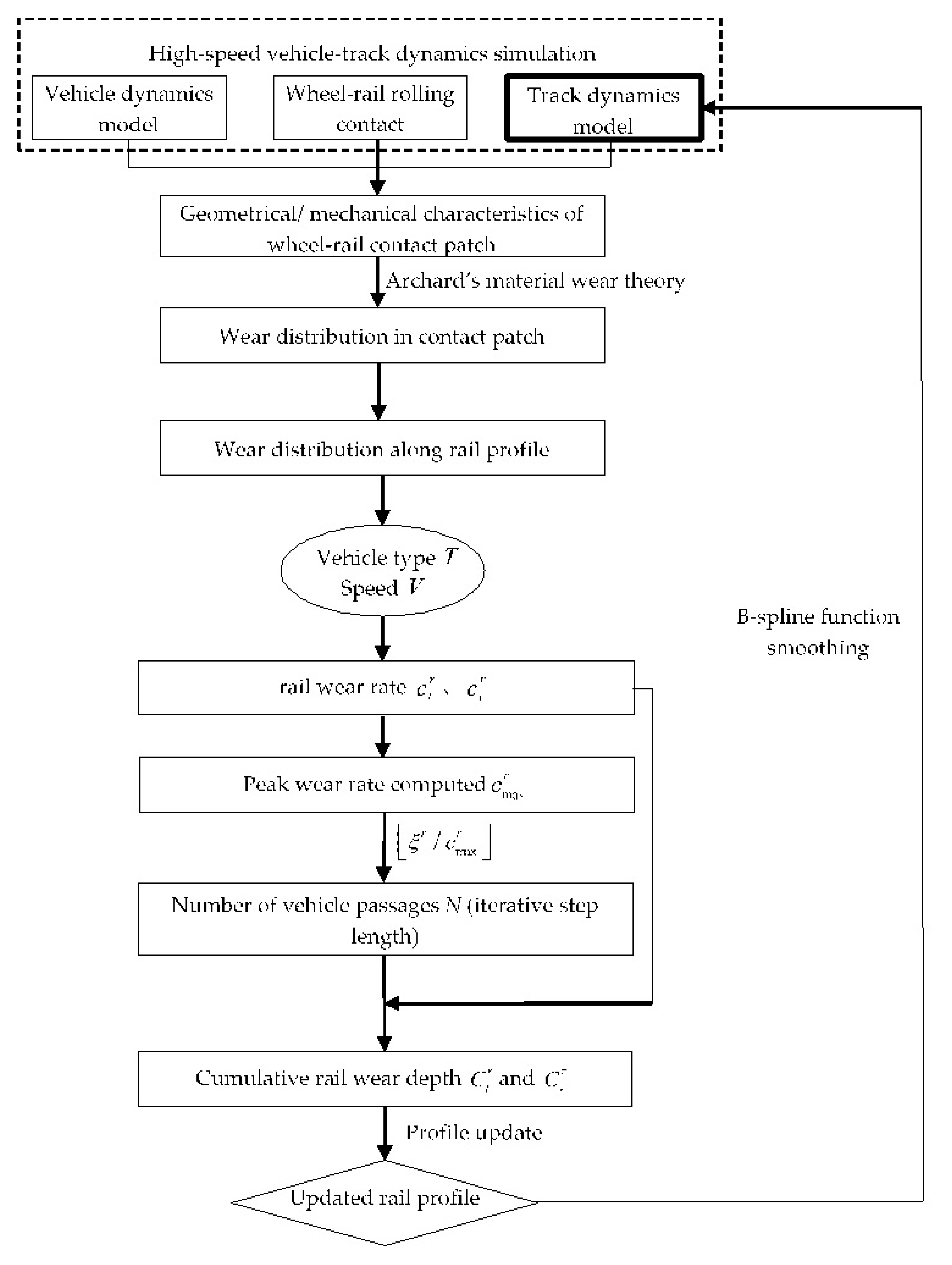
Rail wear originates from wheel–rail interaction dynamics, and the resulting material loss from the rail surface causes changes to the rail profile, which subsequently have a significant impact on the geometric relationship and dynamic interactions between the wheel and the rail. Therefore, rail wear development can be considered a process of interactions during which the rail profile changes in a gradual and continuous manner. Numerical simulation methods are incapable of simulating a continuously changing process; hence, discretization is necessary. Considering this, the rail wear development process was taken as a series of discrete steps, and iterative computation was used by assuming the rail profile remains unchanged and the changes in dynamic wheel–rail behavior resulting from rail profile changes are negligible within each iterative step. In this manner, the wear development was simplified to a linear change occurring within each iterative step. At the end of each iterative step, the cumulative rail wear was computed according to the wear rate and step length, and the rail profile was updated and input into the next step of the iterative computation as the initial profile. Here, an adaptive step length algorithm was used for the rail profile update in which each iterative step was terminated and the profile was updated when the peak cumulative rail wear value reached a certain limit. The step length was continuously adjusted according to the wear rate in each step. This adaptive step length provides an effective strategy to reduce cumulative errors and improve the reliability and stability of the numerical model.
Figure 13 shows a flowchart of the rail wear development simulation program, providing a clear overview of the entire computation process.
Figure 12 shows the process of wear development simulation calculation. Comparatively, the existing vehicle–track coupling dynamics simulation can only qualitatively simulate the wheel–rail wear. However, to simulate the increasing rail wear material loss and gradually changing rail profile, it is necessary to establish the model described in this paper for calculation. The advantage of this wear model is that it can simulate the concrete change process of rail surface material loss and profile during long-term operation.
Based on the established rail wear simulation model, the influence of the gage widening value on the wear of three curve rails with radii of 250, 300, and 350 m was calculated. The calculated working conditions are listed in Table 18. The speeds of the vehicle passing through the curves were 45, 50, and 55 km/h, the superelevation values of various radius curves were set according to the balanced superelevation, the gage widening amount was increased from 0 to 20 mm, and the value interval was 5 mm. The wheels were LM treads, the rail was 60 kg/m, and the rail bottom slope was 1/40. The wear of the rail in the circular curve section under the condition of a total weight of 15 MGT was analyzed.
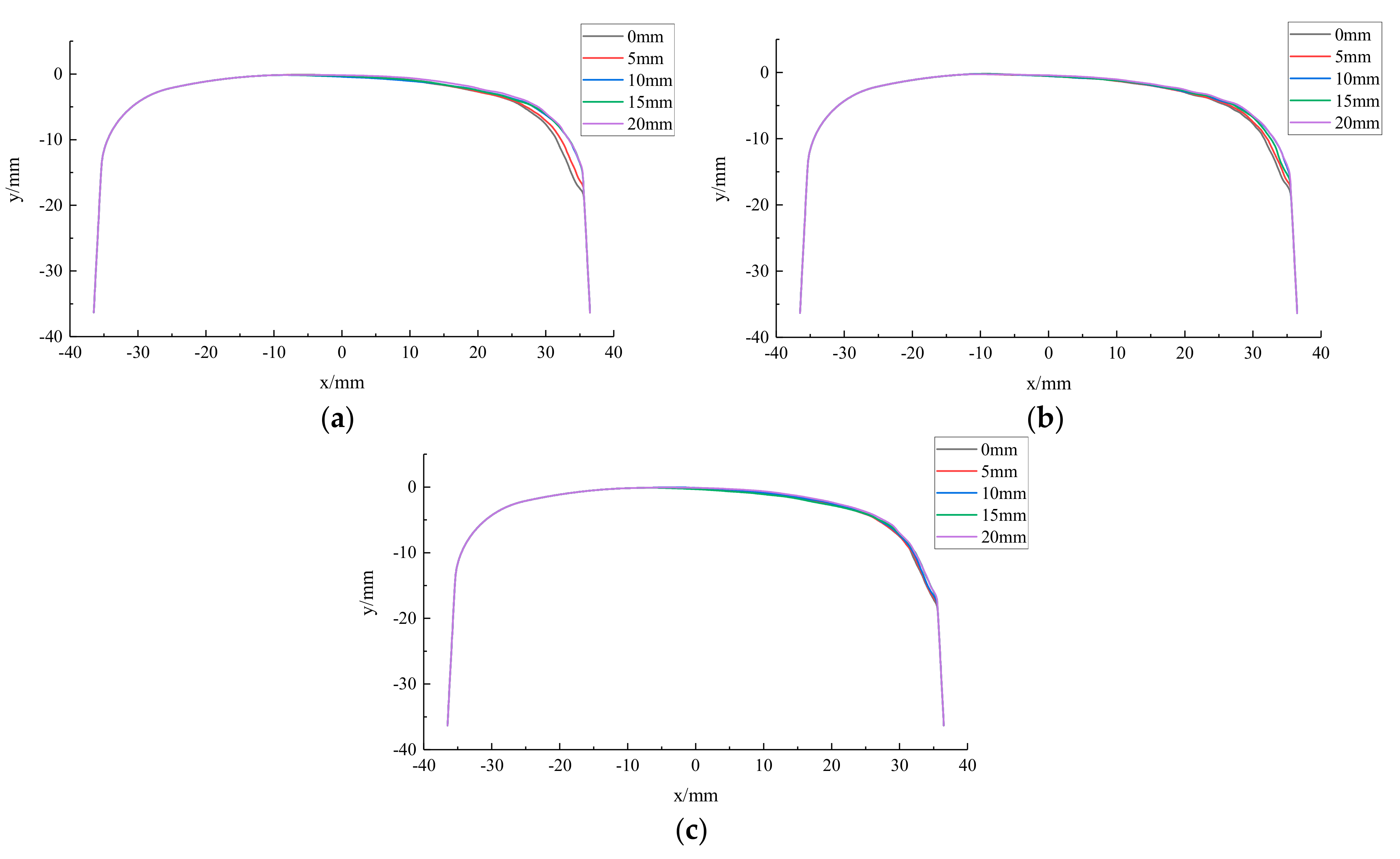
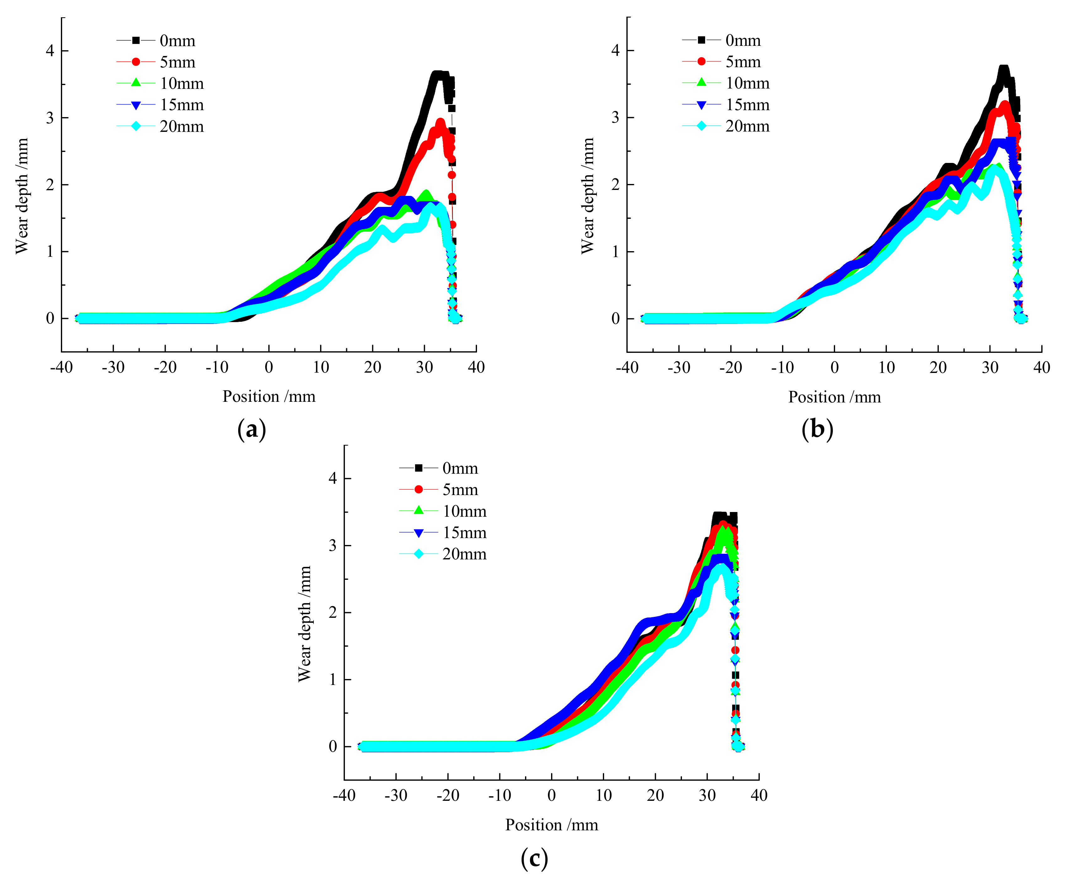
Figure 14 and Figure 15 show the evolution regularity and main wear areas, respectively, of rail profiles with different radius curves. Under various gage widening conditions, the rail wear area is distributed in three areas: the rail side, rail shoulder, and rail top. The rail side area has the largest wear value, the rail side having the second, and the rail top, the smallest.
Considering the maximum wear value as the analysis object, the influence regularity of the gage widening value on rail wear was studied, as shown in Figure 16. With the increase in the gage widening value, the wear amount exhibits a downward trend. The wear amount of a curved rail with a radius of 350 m was reduced from 3.65 to 1.67 mm, the wear amount of a curved rail with a radius of 300 m was reduced from 3.73 to 2.23 mm, and the wear amount of a curved rail with a radius of 250 m was reduced from 3.45 to 2.66 mm. When the gage widening value increased from 0 to 10 mm, the wear amount rapidly decreased. When the gage widening value exceeded 10 mm, the rate of rail wear continued to decrease, and the change in rail wear gradually stabilized, which is consistent with the dynamics calculation results presented in Section 4.1.
4.3. Influence of Gage Widening on Maintenance Workload
On 22 November 2019, we communicated with the Shijiazhuang Section of the Beijing Railway Bureau to understand the use and maintenance situation of the Shijiazhuang–Taiyuan Railway. The Shijiazhuang–Taiyuan Railway is mainly used for freight cars, with only a few regular-speed passenger cars. Heavy trucks run on the upline, and empty trucks run on the downline. The annual transportation volume of the upline is about 140 million tons. The length of the Shijiazhuang–Taiyuan Railway in the Shijiazhuang section is 117 km. The main line contains 149 small-radius curves with a radius of smaller than 400 m (75 upline and 74 downlines). Table 19 lists the distribution of curves with different grades of radius, wherein majority curves have a radius of 300 m or smaller, constituting over 60% of the total radii, whereas the smallest radius is 278 m. According to the current gage widening standard, six curves need to be widened: three uplines and three downlines.
As the rails in the curve section with a radius of 300 m or below cannot be polished by a polishing train, the upper strand side of the rail is severely worn, and the lower strand is collapsed and deformed into a flat shape, accompanied by obvious peeling pieces, as shown in Figure 17. The severe wear and contact fatigue caused the rail life to be considerably reduced. Table 20 lists the rail life statistics results. The downline mainly runs empty cars, and the rail life generally exceeds six years. The life of the rails on the upline is significantly lower. When the radius range is the same, the U78CrV heat-treated rail is significantly longer than the U75V heat-treated rail. Replacing rails has become the primary task, which requires substantial labor and material resources. Owing to the limited number of personnel in the work areas, guaranteeing daily inspection and maintenance is difficult.
According to the current gage widening standard, curves with radii less than 295 m should be widened. Most of the curves on the Shijiazhuang–Taiyuan Railway do not need to be widened. The maintenance regulations stipulate that the gage limit for temporary repairs should not exceed 16 mm. It is known that both rail wear and fastener structure deformation cause the gage to expand. When the rail side wear reaches 10–11 mm, the gage usually reaches 1450 mm. At this time, the work department restores the gage to 1435 mm; when the rail wear reaches the limit value of 19 mm, the rail is replaced. Therefore, the rail gage needs to be adjusted once in the lifecycle of the rail. The rail maintenance process is shown in Figure 18a. The gage varies in the range of 1435–1450 mm, the average gage is 1442.5 mm, and the equivalent widening amount is 7.5 mm.
According to the original gage widening standard (before 2014), the gage should be widened if the radius is less than 350 m. The small radius of the Shijiazhuang–Taiyuan Railway would need to be widened by 5 mm, and the nominal gage size is 1440 mm. According to on-site maintenance and repair experience, when the rail side wore 6–7 mm, the gage would reach 1450 mm; at this time, the work department would restore the gage to 1440 mm; when the wear reached 12–13 mm, the gage expanded to 1450 mm, and the gage would be adjusted again to 1440 mm; when the wear amount reached 19 mm, the rail would have been replaced with the lower track. Therefore, adjusting the gage twice during the lifecycle of the rail is necessary. The maintenance process of the rail is shown in Figure 18b. It can be seen that the gage varies in the range of 1440–1450 mm, the average gage is 1445 mm, and the equivalent widening amount is 10 mm.
Compared with the original gage widening standard, the implementation of the current gage widening standard can reduce the workload of gage adjustment.
5. Conclusions and Recommendations
Based on the analysis of the theory of gage widening for small-radius curves in China and abroad, we examined gage widening standards in various countries and adopted dynamics theory to calculate the influence of gage widening on the curve passing performance. The conclusions and recommendations are provided as follows.
- The existing gage widening theory can determine the minimum curve radius that needs to be widened and the gage widening value required for curves with different radii to ensure that the vehicle passes through the curves in a free-inscribed state. The theory can also determine whether multiaxle locomotives can pass a small-radius curve in a normal forced manner. The theory assumes that the bogie is a rigid structure and that the wheel sets and bogies do not produce turning angles; however, it does not consider the wheel–rail creepage guiding function and the turning resistance of the car body to the bogie. Therefore, the calculation theory of gage widening is conservative, and the influence of the gage widening value on the curve passing performance and track maintenance workload cannot be quantified.
- The minimum curve radius that needs to be widened is 220–350 mm; however, some countries adopt 600 m. The maximum gage widening amount range is 15–20 mm, and only few countries adopt values exceeding 30 mm. China’s gage widening standards are equivalent to those commonly used abroad.
- Dynamics and wear models were established to analyze the influence of the gage widening value on the curve passing performance and rail wear. The calculation results showed that when the gage widening value is increased from 0 to 10 mm, the lateral force of the curved wheel–rail with a radius less than 300 m is reduced by 16–20% and that with a radius exceeding 300 m is reduced by 10–15%. When the gage widening amount exceeds 10 mm, the wheel–rail lateral force tends to be stable, and the rail wear exhibits a similar trend. Therefore, appropriately setting the gage widening value can reduce the wheel–rail lateral force and improve curve passing performance. However, after the gage widening reaches certain values, the effects of improvement will not be apparent.
- Research on the maintenance and repair of the small-radius curves of the Shijiazhuang–Taiyuan Railway showed that the replacement of the small-radius curve rail and the adjustment of the gage are primary maintenance tasks. In the rail lifecycle, the implementation of the current gage widening standard requires only one gage adjustment operation, whereas the implementation of the original gage widening standard requires doubling gage adjustment operations.
Based on the simulation results and field maintenance investigation, it is better not to modify the existing gage widening standards. However, further research is still needed. The gage widening value, wheel–rail profile matching, superelevation setting, and lubrication all affect curve passing performance, and rails with small-radius curves have high wear rates and fast plastic deformation. To further analyze the influence of gage widening on rail life and track maintenance workload, we recommend establishing testing and comparison sections for long-term observation and dynamic testing. At present, we are conducting related tests on the Shuozhou–Huanghua Railway. After selecting specific test sections, we gradually adjust the value of widening small radius curves, conduct dynamic tests, observe wear development, investigate service life and maintenance workload, study the influence pattern of widening small radius curves, and check against simulation analysis. In addition, the study in this paper was mainly based on new wheels. In actual line operations, there are wheels passing through curve sections under different wear conditions. At the same time, with increasing operation time, the rail wear in curve sections continues to develop and change. In the next step, the effect of slight radius curve widening will be studied under various wheel wear conditions.
Author Contributions
P.W.: methodology, funding acquisition, writing—original draft. D.S.: conceptualization, formal analysis, validation. S.W.: investigation, writing—review and editing. Q.Y.: software. All authors have read and agreed to the published version of the manuscript.
Funding
This research was funded by the National Natural Science Foundation of China, grant numbers 51808557 and51878661.
Institutional Review Board Statement
Not applicable.
Informed Consent Statement
Not applicable.
Data Availability Statement
Not applicable.
Conflicts of Interest
The authors declare no conflict of interest.
References
- El Beshbichi, O.; Wan, C.; Bruni, S.; Kassa, E. Complex eigenvalue analysis and parameters analysis to investigate the formation of railhead corrugation in sharp curves. Wear 2020, 450–451, 203150. [Google Scholar] [CrossRef]
- Wang, J.; Chen, X.; Li, X.; Wu, Y. Influence of heavy haul railway curve parameters on rail wear. Eng. Fail. Anal. 2015, 57, 511–520. [Google Scholar] [CrossRef]
- Zboinski, K.; Golofit-Stawinska, M. Investigation into nonlinear phenomena for various railway vehicles in transition curves at velocities close to critical one. Nonlinear Dyn. 2019, 98, 1555–1601. [Google Scholar] [CrossRef] [Green Version]
- Real, T.; Hernandez, C.; Ribes, F.; Real, J.I. Structural and dynamic performance of an asphalt slab track in a sharp curve. KSCE J. Civ. Eng. 2016, 21, 315–321. [Google Scholar] [CrossRef]
- Wang, S.; Zeng, S. Analysis of track capability for curve of motor train unit in Beijing-Tianjin railway line. J. Railw. Eng. Soc. 2007, S1, 195–200. [Google Scholar]
- Chen, R.; Wen, J.; Yu, H.; An, B.; Xu, J.; Wang, P. Influence of rail gauge on wheel-rail contact behavior of metro line. J. Cent. South Univ. Sci. J. 2020, 51, 824–831. [Google Scholar]
- Wu, Z. Calculation basis of the standard of widening gauge for small-radius curve in railway of metallurgical enterprise. Angang Tech. 1983, 38–41. [Google Scholar]
- Zeng, Y.; Zhong, G.; Yang, C. Analysis of gauge widening in small radius curve section of meter-gauge railway. Railw. Constr. Technol. 2020, 48–52. [Google Scholar]
- Chen, P.; Liu, X.; Zhang, Z.; Ma, S.; Chen, Z. Analysis on wheel rail contact in curve section of heavy haul railway. Railw. Eng. 2020, 60, 123–127. [Google Scholar]
- Zhong, Z. Study on Rail Wear in Small-Radius Curve of Heavy-Haul Railway; Beijing Jiaotong University: Beijing, China, 2014. [Google Scholar]
- Conell, W.E. Track gauge and flangeway widths for operation of diesel power on curved track. Area Bull. 1958, 59, 1011–1017. [Google Scholar]
- Bettaieb, H. Analytical dynamic and quasi-static model of railway vehicle transit to curved track. Mech. Ind. 2012, 13, 231–244. [Google Scholar] [CrossRef]
- Zhang, Z. Widening the gauge in curve of railway. Strip Coal Min. Technol. 1994, 46–47. [Google Scholar]
- Hou, F.; Zeng, S. Research gauge widening condition in curve section on Beijing-Tianjin passenger dedicated railway line. Railw. Eng. 2006, 46, 98–100. [Google Scholar]
- Feng, Z. Simulation research on operation safety of EMU negotiating small radius curve. China Railway Science. 2017, 38, 9–15. [Google Scholar]
- Nielsen, J.; Igeland, A. Vertical dynamic interaction between train and track influence of wheel and track imperfections. J. Sound Vib. 1995, 187, 825–839. [Google Scholar] [CrossRef]
- Lu, X. Discussion on maintenance standard of railway. Railw. Eng. 1982, 22, 31–34. [Google Scholar]
- Wei, Z.; Zhang, Z.; Gai, Y. Calculation of gauge widening in curve of mine railway. Min. Process. Equip. 2007, 35, 70–71. [Google Scholar]
- He, Y.; McPhee, J. Optimization of curving performance of rail vehicles. Veh. Syst. Dyn. 2005, 43, 895–923. [Google Scholar] [CrossRef]
- Zeng, S. Gauge widening in curve of railway. Railw. Eng. 1978, 18, 17–21. [Google Scholar]
- Zeng, S.; Luan, C. Study on gauge widening in curve of railway. J. China Railw. Soc. 1981, 3, 77–88. [Google Scholar]
- China Railway Corporation. Rules for Maintenance of Railway; China Railway Publishing House: Beijing, China, 2019. [Google Scholar]
- China Railway Corporation. Regulations for Railway Technical Management; China Railway Publishing House: Beijing, China, 2014. [Google Scholar]
- Adachi, M.; Matsumoto, A. Improvement of curving performance by expansion of gauge widening and additional measures. Proc. Inst. Mech. Eng. Part F J. Rail Rapid Transit 2012, 226, 203–215. [Google Scholar] [CrossRef]
- Popović, Z.; Lazerević, L.; Vatin, N. Analysis of Track Gauge Widening in Curves with Small Radius. Appl. Mech. Mater. 2015, 725–726, 967–973. [Google Scholar] [CrossRef] [Green Version]
- Wang, J.; Li, Y. Research on the widening track gauge and structure gauge of railway turnout. J. Railw. Eng. Soc. 2009, 26, 20–22. [Google Scholar]
- Novikov, V.; Panchenko, S.; Skoryk, O. Investigation into the conditions causing terminal-bolted track gauge widening and consideration of it in the critical gauge calculation. Collect. Sci. Work. Ukr. State Univ. Railw. Transp. 2018, 14–20. [Google Scholar] [CrossRef]
- Pyrgidis, C. Calculation of the Gauge Widening of a Track with the Aid of Mathematical Models. In Proceedings of the 8th International Conference on Maintenance & Renewal of Permanent Way, Power & Signalling, Structures & Earthworks 2005, London, UK, 29–30 June 2005. [Google Scholar]
- Vineesh, K.; Vakkalagadda, M.; Dev, M.; Rao, B.; Racherla, V. Gauge widening of passenger coach wheel sets in Indian Railways: Observed statistics and failure analysis. Eng. Fail. Anal. 2017, 71, 105–119. [Google Scholar] [CrossRef]
- Kamaitis, I.Z.; Podagėlis, I.; Povilaitiene, I. Durability of Rails on Track Curves. In Proceedings of the IABSE Conference: Role of Structural Engineers towards Reduction of Poverty, New Delhi, India, 19–22 February 2005; pp. 349–355. [Google Scholar]
- Vakkalagadda, M.; Vineesh, K.; Mishra, A.; Racherla, V. Locomotive wheel failure from gauge widening/condemning: Effect of wheel profile, brake block type, and braking conditions. Eng. Fail. Anal. 2016, 59, 1–16. [Google Scholar] [CrossRef]
- Wang, W.; Luo, X. Metro gauge widening in transition section with transition curve. Urban Rapid Rail Transit 2015, 28, 60–64. [Google Scholar]
Figure 1.
Schematic of the geometrically free-inscribing method.

Figure 2.
Schematic of the dynamically free-inscribing method.

Figure 3.
Gap calculation based on dynamically free inscribing.

Figure 4.
Schematic of the wedge-shaped inscribing method.

Figure 5.
Schematic of gage widening calculations utilized in Japan.

Figure 6.
Schematic of the topological structure of the truck dynamics model.

Figure 7.
Track dynamics model.

Figure 8.
Fastener system model.

Figure 9.
Schematic of rail tipping.

Figure 10.
The influence of the gage widening value on wheel or rail lateral force. (a) R150 m; (b) R200 m; (c) R250 m; (d) R300 m; (e) R350 m; (f) R400 m.
Figure 10.
The influence of the gage widening value on wheel or rail lateral force. (a) R150 m; (b) R200 m; (c) R250 m; (d) R300 m; (e) R350 m; (f) R400 m.

Figure 11.
Wear calculation model.

Figure 12.
Diagram of superposition of rail profile wear.

Figure 13.
Iterative computation process for numerical prediction of rail wear development.

Figure 14.
Evolution regularity of the rail profile. Radius: (a) 350 m; (b) 300 m; and (c) 250 m.

Figure 15.
Rail wear area. Radius: (a) 350 m; (b) 300 m; and (c) 250 m.

Figure 16.
Influence of gage widening on rail wear amplitude: (a) 350 m; (b) 300 m; and (c) 250 m.


Figure 17.
Surface damage situation of a small-radius-curve rail. (a) Upper strand; (b) Lower strand.
Figure 17.
Surface damage situation of a small-radius-curve rail. (a) Upper strand; (b) Lower strand.

Figure 18.
The influence of gage widening on track maintenance and repair. (a) Current gage widening standards; (b) the original gage widening standard.
Figure 18.
The influence of gage widening on track maintenance and repair. (a) Current gage widening standards; (b) the original gage widening standard.


Table 1.
Gage widening values used in the Soviet Union (before 1961).
| Curve Radius (m) | >650 | 650–451 | 450–351 | <350 |
| Widening Value (mm) | 0 | 6 | 11 | 16 |
Table 2.
Rail gage widening value in the former Soviet Union (after 1961).
| Curve Radius (m) | ≥350 | 349–300 | ≤299 |
| Widening Value (mm) | 0 | 6 | 16 |
Table 3.
Rail gage widening value in Russia (Currently used).
| Curve Radius (m) | ≥350 | 349–300 | ≤299 |
| Widening Value (mm) | 0 | 10 | 15 |
Table 4.
Gage widening values used in American railways (mm).
| Curve Radius (m) | ≥219 | 218–195 | 194–175 | 174–159 | 158–146 | 145–134 |
| Widening Value (mm) | 0 | 3.12 | 6.24 | 9.36 | 12.5 | 15.6 |
Table 5.
Gage widening values used in Japanese railways (mm).
| Curve Radius (m) | >600 | 600–440 | 440–320 | 320–240 | 240–200 | 200–170 | ≤170 |
| Widening Value (mm) | 0 | 5 | 10 | 15 | 20 | 25 | 30 |
Table 6.
Gage widening values in West German railways (mm).
| Curve Radius (m) | >200 | 200–172 | 172–150 | 150–134 | 134–100 |
| Widening Value (mm) | 0 | 5 | 10 | 15 | 20 |
Table 7.
Gage widening values in West German railways (mm).
| Curve Radius (m) | >300 | 300–200 | 200–150 | 150–120 | 120–100 |
| Widening Value (mm) | 0 | 5 | 10 | 15 | 20 |
Table 8.
Gage widening values in East German railways (mm).
| Curve Radius (m) | >300 | 299–251 | 250–201 | 200–180 | 180–160 | <160 |
| Widening Value (mm) | 0 | 5 | 10 | 15 | 20 | 25 |
Table 9.
Gage widening values in Chinese railways (1954) (mm).
| Curve Radius (m) | ≥651 | 650–451 | 450–351 | ≤350 |
| Widening Value (mm) | 0 | 5 | 10 | 15 |
Table 10.
Gage widening values in Chinese railways (1954) (mm).
| Superelevation (mm) | Curve Radius (m) | Driving Speed (km/h) | |||||||||
|---|---|---|---|---|---|---|---|---|---|---|---|
| 5 | 20 | 30 | 40 | 50 | 60 | 70 | 80 | 90 | 100 | ||
| 100 | 350 | −3.7 | −4.4 | −4.8 | −5.2 | −5.7 | −6.1 | −6.7 | −7.5 | −8.2 | −9.4 |
| 300 | −1.6 | −2.0 | −2.5 | −3.1 | −3.7 | −4.5 | −5.4 | −6.0 | −7.5 | −9.1 | |
| 250 | 1.5 | 2 | 0.4 | −0.4 | −1.2 | −2.0 | −2.9 | −4.5 | −7.2 | −10.5 | |
| 200 | 4.4 | 3.7 | 2.8 | 1.9 | 0.7 | −0.5 | −2.4 | ||||
Table 11.
Gage widening values in Chinese railways (1983) (mm).
| Curve Radius (m) | ≥350 | 350–300 | <300 |
| Widening Value (mm) | 0 | 5 | 15 |
Table 12.
Gage widening values in Chinese railways (1983) (mm).
| Locomotive Type | Number of Axes | Wheelbase | Widening Amount (mm) | 0 | 5 | 10 | 15 |
|---|---|---|---|---|---|---|---|
| FD-type | 5 | 1625 + 1625 + 1625 + 1625 | Minimum Curve Radius (m) | 283 | 209 | 166 | 137 |
| Forward-type | 5 | 1600 + 1600 + 1600 + 1600 | 256 | 192 | 153 | 128 |
Table 13.
Geometrically free-inscribed gage widening values.
| Curve Radius R(m) | Wheelset Width qmax (mm) | Outer Vector Distance f0 (mm) | Gage s (mm) | Gage Widening Amount (mm) |
|---|---|---|---|---|
| 350 | 1422 | 10.4 | 1432.4 | −2.6 |
| 300 | 1422 | 12.2 | 1434.2 | −0.8 |
| 250 | 1422 | 14.6 | 1436.6 | 1.6 |
| 200 | 1422 | 18.2 | 1440.2 | 5.2 |
| 150 | 1422 | 24.3 | 1446.3 | 11.3 |
Table 14.
Minimum curve radii (m) that a locomotive can pass through with normal forced inscribing.
| Gage Widening Amount (mm) | Electric Locomotive | Diesel Locomotive | Steam Locomotive |
|---|---|---|---|
| 0 | 93.5 | 101.7 | 126.5 |
| 5 | 90.9 | 99.2 | 122.1 |
| 10 | 88.4 | 96.9 | 118.1 |
| 15 | 86.0 | 94.7 | 114.3 |
Table 15.
Current gage widening values (mm).
| Curve Radius (m) | R ≥ 295 | 295 > R ≥ 245 | 245 > R ≥ 195 | R < 195 |
| Widening Value (mm) | 0 | 5 | 10 | 15 |
Table 16.
Calculated working conditions.
| Radius (m) | Superelevation (mm) | Speed (km/h) |
|---|---|---|
| 150 | 36 | 35 |
| 96 | ||
| 156 | ||
| 200 | 34 | 40 |
| 94 | ||
| 154 | ||
| 250 | 35 | 45 |
| 95 | ||
| 155 | ||
| 300 | 38 | 50 |
| 98 | ||
| 158 | ||
| 350 | 42 | 55 |
| 102 | ||
| 162 | ||
| 400 | 46 | 60 |
| 106 | ||
| 166 |
Table 17.
Wear coefficient .
| 1 × 10⁻⁴ ~ 10 × 10−4 | 30 × 10−4 ~ 40 × 10−4 | 1 × 10⁻⁴ ~ 10 × 10−4 | |
| 300 × 10−4 ~ 400 × 10−4 | |||
Table 18.
Rail wear simulation conditions.
| Curve Radius (m) | Speed (km/h) | Outer Rail Superelevation (mm) | Gage Widening Value (mm) |
|---|---|---|---|
| 250 | 45 | 95 | 0 |
| 5 | |||
| 10 | |||
| 15 | |||
| 20 | |||
| 300 | 50 | 98 | 0 |
| 5 | |||
| 10 | |||
| 15 | |||
| 20 | |||
| 350 | 55 | 102 | 0 |
| 5 | |||
| 10 | |||
| 15 | |||
| 20 |
Table 19.
Distribution of curves.
| Radius | Upline | Downlines |
|---|---|---|
| 350 < R ≤ 400 | 6 | 7 |
| 300 < R ≤ 350 | 24 | 19 |
| R ≤ 300 | 45 | 48 |
Table 20.
Statistical results on curved rail life (years).
| Radius | Upline | Downline | ||
|---|---|---|---|---|
| U78CrV | U75V | U78CrV | U75V | |
| 350 < R ≤ 400 | 3.42 | 2.67 | 9.64 | 9.57 |
| 300 < R ≤350 | 3.33 | 2.4 | 8.07 | 7.41 |
| R ≤ 300 | 2.42 | 1.34 | 7.61 | 6.2 |
Publisher’s Note: MDPI stays neutral with regard to jurisdictional claims in published maps and institutional affiliations. |
© 2021 by the authors. Licensee MDPI, Basel, Switzerland. This article is an open access article distributed under the terms and conditions of the Creative Commons Attribution (CC BY) license (https://creativecommons.org/licenses/by/4.0/).
Share and Cite
MDPI and ACS Style
Wang, P.; Si, D.; Wang, S.; Yi, Q. Study on Gage Widening Methods for Small-Radius Curves. Appl. Sci. 2021, 11, 5334. https://doi.org/10.3390/app11125334
AMA Style
Wang P, Si D, Wang S, Yi Q. Study on Gage Widening Methods for Small-Radius Curves. Applied Sciences. 2021; 11(12):5334. https://doi.org/10.3390/app11125334
Chicago/Turabian StyleWang, Pu, Daolin Si, Shuguo Wang, and Qiang Yi. 2021. "Study on Gage Widening Methods for Small-Radius Curves" Applied Sciences 11, no. 12: 5334. https://doi.org/10.3390/app11125334
Note that from the first issue of 2016, this journal uses article numbers instead of page numbers. See further details here.