Transient Effects in Atmosphere and Ionosphere Preceding the 2015 M7.8 and M7.3 Gorkha–Nepal Earthquakes

Introduction

The observational evidence of data from the last 3 decades from different parts of the world provides a significant pattern of transient anomalies preceding earthquakes (Tronin et al., 2002; Liu et al., 2004; Ouzounov et al., 2007; Nĕmec et al., 2008; Parrot, 2009; Kon et al., 2010; Hayakawa et al., 2013; Tramutoli et al., 2013). Although there exists a great deal of experimental evidence on the presence of seismo-electromagnetic disturbances in the wide frequency range from Ultra Low to High Frequency and methods of observations stretch out from ground to satellite (Pulinets and Boyarchuk, 2004; Hayakawa 2015; Ouzounov et al., 2018a), the majority of the studies presented were obtained at one location, one wave path or only at the time of the events. It is rare to see “aseismic path” measurements, i.e., data from the receivers (or outfit) located far away from the earthquake epicenters. Long-term statistical analysis, or confutation analysis for other possible causes needs to be explored, which can produce the same signal anomalies. Sometimes there are demonstrations only on a single parameter and therefore many researchers have rational skepticism about pre-earthquake anomalies. We focus on the consistent multi-parameter data collection that could help to reveal the connection between atmospheric and ionospheric variations (or anomalies) associated with major earthquakes.

The 2015 earthquake sequence in Nepal has been studied with different methods for pre-earthquake anomalies. Several authors show precursory phenomena by using different satellite and ground observations: a/Satellite thermal anomalies (Ouzounov et al., 2015; Prakash et al., 2015; Shan et al., 2016); b/Microwave Brightness Temperature Anomalies (Qi et al., 2020); c/Radon anomalies (Deb et al., 2016); d/Ionospheric anomalies (Ouzounov et al., 2015; Maurya et al., 2016; Oikonomou et al., 2016; Li et al., 2016; De Santis et al., 2017); e/Gravity anomalies (Chen et al., 2015). We used a multi-parameter approach to search for pre-earthquake signals associated with the series of strong earthquakes in Nepal during April-May 2015. A network of different observations provides an opportunity to analyze signals over the same area with different methods. Our study analyzed ground and satellite data to record the atmospheric and ionospheric responses to the M7.8 and M7.3 earthquakes in Nepal in 2015. Immediately after the M7.8 on April 25, 2015, we could analyze and find anomalies in the atmosphere prospectively and acknowledge in advance the potential for the occurrence of M7.3 of May 12, 2015 (Ouzounov et al., 2015). We examined six different physical parameters characterizing the state of the atmosphere/ionosphere during the periods before and after the event: 1. Outgoing Longwave Radiation, OLR (infra-red 10–13 µm) measured at the top of the atmosphere; 2. GPS/TEC (Total Electron Content) ionospheric variability; 3. Very Low Frequency (VLF) over horizon propagation; 4. Radon observations; 5. Atmospheric chemical potential from assimilation models and 6. Air Temperature from NOAA ground stations. These results testify to the efficiency of combining different methods (Thermal, GPS/TEC, VLF/LF) for the revealing precursory activity associated with strong earthquakes, especially with multi-stationed observations.

Earthquakes

The Nepal earthquake on April 25 was the strongest since 1934. The Mw = 7.8 (depth 15 km) earthquake with epicenter 28.230°N, 84.731°E occurred in the same area at 06:11 UT, 80 km from Kathmandu. A series of strong aftershocks began immediately after the mainshock, with one aftershock reaching Mw = 6.6 (depth = 10 km) within half an hour of the initial earthquake. A major aftershock of Mw = 6.9 occurred on April 26, 2015, in the same region at 07:08 UT. The weaker aftershocks were observed until the morning of April 28. According to the USGS, the earthquake was caused by a sudden thrust, or release of built-up stress, along the primary fault line where the Indian Plate is slowly diving underneath the Eurasian Plate, carrying much of Europe and Asia. The earthquake’s effects were amplified in Kathmandu as it sits in the Kathmandu Basin, which contains about 600 m of sedimentary rocks, representing the infilling of an ancient lake.

Kathmandu, situated on a block of the crust of approximately 120 km wide and 60 km long, reportedly shifted 3 m to the south in a matter of just 30 s. This earthquake caused avalanches on Mount Everest. At least 19 people died, with 120 others injured or missing (Harris, 2015). In total there have been more than 8,669 victims and 17866 injured. Tens of hundred houses were destroyed, including several pagodas on Kathmandu Durbar Square (a UNESCO World Heritage Site) and the 60-m tower Dharahara. More than half a million structures were damaged. The second Nepalese earthquake occurred on May 12, 2015, at 07:05 UT with Mw = 7.3 (depth 18 km). This earthquake occurred on the same fault as the April 25, but further east than the original earthquake. Minutes later, another 6.3 magnitude earthquake hit Nepal, with its epicenter east of Kathmandu. The tremor caused new landslides and avalanches on Mount Everest and was felt at many places in northern India. It destroyed some of the buildings which survived the first earthquake. (Figure 1).

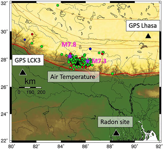
FIGURE 1. Reference map of Nepal region, with the location of earthquakes >M4 for Jan–May 2015. The location of M7.8 of April 25 and M7.3 of May 12, 2015 are with purple stars. With black triangles are showing the location of the air Temperature station (katmandu) and GPS stations (Lhasa), radon site (Kolkata, India).

Results

Air Temperature Observations

Multiyear day-by-day counts of nighttime temperatures were used to compute the daily temperature variations near the vicinity of the earthquake epicenter. Data near the ground surface were obtained from Tribhuvan International Airport, Nepal, through NOAA Surface Data Hourly Global Database. We analyzed surface air temperature and nighttime data for 2011–2015 close to the terminator time 0,500–0,600 LT to define the normal and abnormal state of the air temperature. The pre-terminator times have been found as one of the most sensitive indicators for buildup of thermal anomalies, because of the limited solar radiation impact during these hours (Ouzounov et al., 2006). The time series for January 1 to May 31, 2015, is shown in Figure 2C. We computed the residual values to distinguish between the current value and the multi-year year mean of the air temperature variability. The maximum offsets from the mean value reached near +5°C on April 20 and +4°C on May 5 (Figure 2C) with a confidence level of more than +2 sigma for all the observations from 2011 to 2015. This transient rapid increase in the surface air temperature is a little more significant than the remote satellite observations shown in Figure 2A, which agrees with the thermodynamic processes explained by the LAIC concept. (Pulinets and Ouzounov, 2011). To understand the day-by-day variability of the daytime and nighttime temperature during the earthquake events, we analyzed the hourly temperature near the epicenter in a new way. We used 3-h global surface air temperature data from the GEOS-5 assimilation (Figure 2B). The presence of ions in the atmosphere creates a possibility for water vapor molecules to join with these ions through the hydration process, which is different from condensation. The evaporation/condensation process, the phase transition of the first order, always occurs during the potential chemical equality. However, newly formed ions have different chemical potentials; what is to introduce should consider in the one-component approximation we introduce the correction to the chemical potential. The increase of the water molecules chemical potential indicates the strength of the nucleation process and can be used as an indicator of an imminent earthquake according to Boyarchuk et al., 2010 and demonstrated already within multiparameter analysis (Ouzounov et al., 2018a; Pulinets et al., 2020).

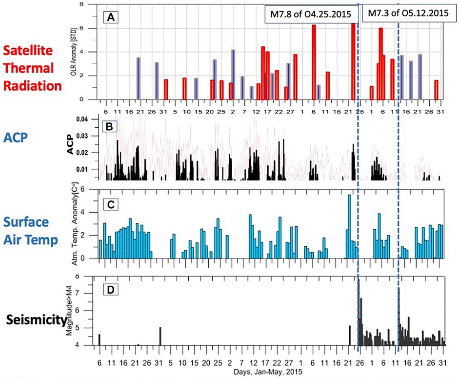
FIGURE 2. Time series of atmospheric variability observed within a 200 km radius of the Nepal earthquake (top to bottom): (A) Nighttime anomalous OLR over epicentral region from January 1–May 30, 2015 observed from NOAA AVHRR (red). Same location, same period a year before - Jan-Ma y 20 14 (black); (B) ACP time series over the epicentral areas. With pink color 2015 ACP 6 hourly data. With black the residual of 2015-20 14 6 hourly ACP data; (C) Air temperature anomaly from station Tribhuvan International Airport (blue) at 0600LT; (D) Seismicity (M>4.0), Jan–May 2015 within 200km radius of the M 7.8 epicenter (USGS).

Radon Observation

Long-term array observations of radon anomalies have been used for pre-earthquake studies (Fu et al., 2011, 2015, Zoran et al., 2012; Giuliani et al., 2013, Karastathis et al., 2019). Anomalous radon variations occurred a few days to a few months before the earthquake and are likely to be associated with earthquake development’s dilatancy and micro fracturing stages. Radon plays a crucial role in developing the lithosphere-atmosphere-ionosphere coupling (LAIC) concept (Scholz et al., 1973; Pulinets and Ouzounov, 2011; Pulinets et al., 2018) associated with the pre-earthquake process. During the 2015 earthquake sequences in Nepal, simultaneous measurements of soil radon-222 were recorded at the main campus of Jadavpur University, Kolkata, India. Deb et al. (2016) studied the precursory seismogenic radon. To observe coherent responses, the soil Rn222 concentration profiles were measured simultaneously at two nearby (∼200 m apart) locations (Figure 3A), A and B, having uniformly clayey soil, within the Jadavpur University premises (22.5667^◦N, 88.3667^◦E). The soil moisture content at location A was lower than location B. It was expected that simultaneous recording of radon time series at these two locations would add confidence in identifying pre-seismic responses (Figure 3b). The 4-months time of their observations fortunately overlapped with the Nepal seismo-active period in 2015 (Figure 3). Their sensor, a solid-state nuclear track detector method, was used to detect the alpha-radiation in the radioactive radon gas. Two simultaneous 4-months of observations have been analyzed. During the observation period, four statistically significant anomalies (above the ±2σ level) were obtained on April 20, April 29, May 19, and May 29, 2015, simultaneously at both locations A and B. April 20 anomaly preceded the April 25 M7.8, and the April 29 was identified as precursors to the May 12. The May 29 radon anomaly is likely to be identified as a pre-seismic event to the M5.6 earthquake at Kokrajhar, Assam, on June 28, 2015 (Day et al. l, 2016). Despite that radon fluctuation on May 19 registered at locations A and B with >2σ significance, no earthquake occurred within a 1,000 km radius from Kolkata. Probably this anomaly is not associated with seismic origin but with geodynamics transition associated with the new Moon event on May 18, 2015, 1 day before the Radon anomaly occurrence. The connection between Lunar phases, geodynamics, and seismicity has been statistically established (Kolvankar et al., 2010). The overall interpolation of radon anomalies related to the Nepal 2015 earthquakes demonstrates that the reliable detection of radon anomaly due to seismicity requires simultaneous measurement of soil radon concentration by a broad network of radon/gamma sensors (Fu et al., 2011, 2015; Karastathis et al., 2019).

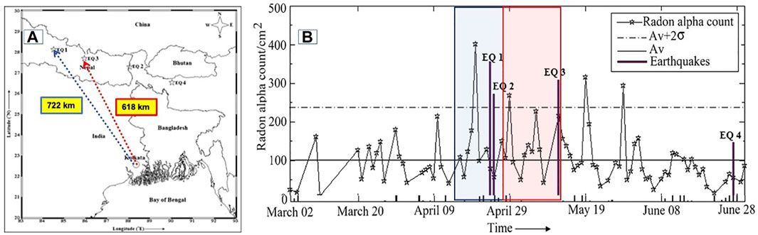
FIGURE 3. Radon observation in Kolkata, India (A) Map indicating the monitoring sites in Kolkata and the MS+ earthquakes within 1000 km region. (B) Combined graph for radon-222 anomalies at location (A) and the corresponding earthquakes during the observation period from March 1 to June 30, 2015. EQ l -M7.8 of 04.25.2015; EQ2- M6.9 of 04.26.2015 and EQ3- M7.3 of OS.12.2015. (Deb at all, 2016).

Atmospheric Chemical Potential

All thermodynamic models of the atmosphere, considering the phase transitions of water and latent heat fluxes, operate with latent heat (per mole or molecule) as a constant at a given temperature. It is equal to 0.422 eV per one water molecule. However, if one carefully deals with accurate data, one can often find that violations of the gas equation are observed (inexplicable additional variations in temperature, humidity, and pressure). We approached this phenomenon from a different approach different when studying the processes of ionization of the surface manner layer of the atmosphere by radon, the release of which from the Earth’s crust sharply increases at the final stage of preparation for a strong earthquake. The detailed calculations could be found in Pulinets et al., (2015). Here we discuss the final findings. As it turned out, atmospheric ions formed during the ionization of atmospheric gases by energetic alpha particles emitted by radon during decay become instantly hydrated. Hydration is not equivalent to condensation because the process takes place at any relative humidity level and does not require saturated steam. However, all the same, a phase transition of water molecules from a free to a bound state takes place, and, just as during condensation, latent heat is released. It turned out that the released amount of latent heat is more significant at a high rate of ion production and high concentration of ions than for ordinary condensation. How much larger? For earthquakes, the value ranges from 0.01 to 0.1 eV, i.e., in extreme cases, it can reach about 25% of the latent heat constant. (it’s the difference between the released latent heat during hydration and normal condensation). This difference we call the correction of the chemical potential of the water vapor in the atmosphere. We call it the atmospheric chemical potential (ACP) because, in the act of evaporation/condensation, the energy of the water molecule is equal to its chemical potential. To understand the day-by-day variability of ACP during the earthquake events, we analyzed 3 h global ACP data computed from the GEOS-5 assimilation (Figure 2B).

Earth Radiation Observation

One of the main parameters we used to characterize the Earth’s radiation environment is outgoing long-wave-earth radiation (OLR). OLR has been associated with the top of the atmosphere (TOA) integrating the emissions from the ground, lower atmosphere, and clouds (Ohring G. and Gruber, 1982), and primarily was used to study the Earth’s radiative budget and climate (Gruber and Krueger, 1984; Mehta and Susskind, 1999).

Daily OLR data were used to study the OLR variability in the zone of earthquake activity (Liu, 2000; Ouzounov et al., 2007, 2018b; Xiong et al., 2010). An augmentation in radiation and a transient change in OLR was proposed to be related to thermodynamic processes in the atmosphere over seismically active regions. We can determine the atmospheric anomaly in Euler’s reference frame as a first approximation by subtracting the mean. The average can be defined at the same day each year, local time, and location over 11 years (i.e., more than one solar cycle). The advantage of this approach is its efficiency in the presence of long-term satellite observations. The OLR anomalous variations were defined as an E_index (Ouzounov et al., 2007) as the statically defined maximum change in the rate of OLR for a specific spatial location and predefined times. They have constructed analogously to the anomalous thermal field proposed by (Tramutoli et al., 2005, 2013).

The E_index was defined as statically estimated variability in OLR values for specific locations and periods:

Where: t = 1, K days, (${\text{S}}^{\text{∗}}\left({\text{x}}_{\text{i},\text{j }},{\text{y}}_{\text{i},\text{j }},\text{t}\right)$) is the current OLR and $\overline{{\text{S}}^{\text{∗}}}\left({\text{x}}_{\text{i},\text{j }},{\text{y}}_{\text{i},\text{j }},\text{t}\right)$ is the computed mean of the OLR field, defined for multiple years of observations over the same location and same local time, ${\text{σ}}_{\text{i},\text{j }}$ is the standard deviation of $\text{S}\text{*}$, and K is the total number of analyzed days. We use the Thermal radiation anomaly (TRA) index, a modified version of E_Index (Eq. (1)),

A and B are regional coefficients, A—a mask, mainly defined by the regional seismo-tectonic patterns and TRA appearance frequency (A = 0.1–0.9). B normalizes each of NOAA 15 and 18-time series of OLR data to the same time coverage over 11 years averaging period (B = 1–3.5). The TRA indexes have been processed with additional preprocessing to avoid aliasing short wavelengths and spatial filtering based on a “minimum curvature” algorithm (Ouzounov et al., 2018a). We used OLR data from NOAA’s Advanced Very High-Resolution Radiometer (AVHRR) for satellite thermal analysis over Nepal. The results of the 2015 Nepal earthquake showed that there was a rapid increase in transient infrared radiation in satellite data in mid-March 2015. An anomaly is observed near the epicenter; it peaked around April 4–7, about 2–3 weeks before the M7.8 earthquake (Figure 4, Figure 6). Further analysis revealed another temporary OLR anomaly on May 2–3. The second M7.3 event occurred on May 12, 2015. (Ouzounov et al., 2015). Our results show that long-wave radiation signals associated with earthquake processes were observed near the epicentral regions several days before the corresponding earthquakes. TRA hotspots appeared quickly, remained in the same regions for several hours, and then quickly dissipated. During March-May 2015, about TRA 15 anomalies were detected around the Nepali M7.3 epicentral areas (Figures 5,6). With red dots showing the anomaly locations, the date is given in the text, and a circle shows the confidence area. The centers TRA are computed based on Eqs. (1), (2). The energetic threshold for determining the anomalous patterns was >2.5 sigma STD. TRAs on April 5, 23, and 29 are within the maximum level for the entire period inside the entire region. The possible reason for several TRA’s is the activating of gas releases over Nepal and Central Asia. The triggered ionization inside the ABL generates zones of “thermal-bursts.” The cross-section of several TRA areas probably indicates the spatial clustering of the degassing along joined tectonic lineaments. The appearance of TRA anomalies almost disappears after the May 12 Earthquakes. The spatial distribution indicates a large appearance area, but the distance from the epicenter is allowed inside the Dobrovolsky (Dobrovolsky et al., 1979) and Bowman et al., 1998 area (R = 10^0.43M/R = 10^0.44M), which is about 2,250 km according to Dobrovolsky. This rapid enhancement of radiation could be explained by an anomalous flux of the latent heat over the area of increased tectonic activity. (Pulinets and Ouzounov, 2011, 2018; De Santis et al., 2017). Analogous observations were observed within a few days before the most recent major earthquakes in Japan (M9, 2011), China (M7.9, 2008), Italy (M6.3, 2009), Samoa (M7, 2009), Haiti (M7, 2010), and Chile (M8.8, 2010) (Ouzounov et al., 2011b, c; Pulinets and Davidenko, 2014).

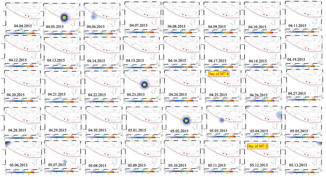
FIGURE 4. Time series of night time TRA observed from NOANAVHRR, April 4–May 13, 2015. Tectonic plate boundaries are indicated with red lines and major faults by brown ones and earthquake location by red circles. Red circles show the spatial location of TRA within vicinity of M7.8 and M7.3.

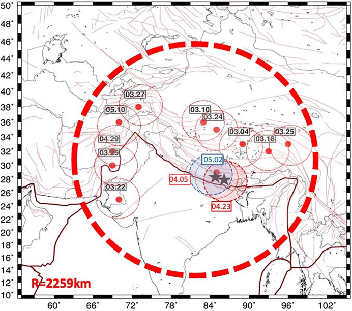
FIGURE 5. Spatial distribution of Thermal Radiation Anomalies (TRA) March-May 2015 and Dobrvolsky estimated area for the earthquake preparation zone (red dash circle). With red shadowed circles 04.03 and 04.23 anomalies. With a blue shadowed circle 05.03.2015 anomaly. With red dots -the centers of TRA anomalies, with dash red circles, the confidence area of TRA. With black stars the epicenters of M7.8 04.25.2015 and M7.3 of05.12.20 15.

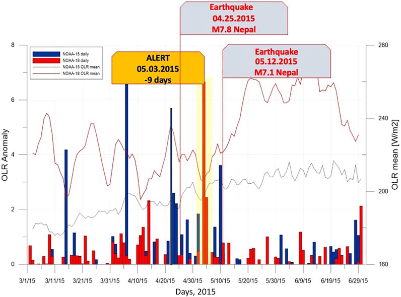
FIGURE 6. TRA time series for March 2015- June 2015 over th’l: e’j\’Jr Gorkha epicentral area. On April 5, 2015 and April 23, were revealed transient anomalies (by retrospective analysis of satellite radiation) 21 and 3 days in advance to the M7.8 mainshock of April 25, 2015, earthquake. On May 3, 2015, the ongoing prospective analysis of satellite radiation revealed transient anomaly (9 days in advance, with yellow), associated with the M7.3 of May 12, 20 15, earthquake.

Pre-seismic Ionospheric Effects

For our analysis of ionospheric data, we used two sources of information: global maps of the total electron content in IONEX format provided by JPL and a time series of calculated vertical TEC of two GPS receivers in the region (lhaz and lck3). We also controlled the solar-geophysical conditions to purify the data from the possible solar-geomagnetic activity effects. Considering that we deal with the equatorial ionosphere, the primary source of geomagnetic activity was the equatorial geomagnetic index Dst provided by Kyoto World Data Center for Geomagnetism (http://wdc.kugi.kyoto- u.ac.jp/dstdir/index.html).

The epicenter of the M7.8 earthquake was at the outer slope of the northern crest of the Equatorial Ionization Anomaly (EIA). To detect the ionospheric precursors, it is necessary to carefully analyze the geophysical conditions around the time of the Nepal earthquakes. For this purpose, the Solar-geophysical conditions during April- May 2015 is shown in Figure 7, where the Solar radio flux F10.7 were analyzed. To put all parameters together (which are expressed in different values), all parameters were normalized. Where F10.7—it is Solar electromagnetic radiation on the Wavelength 10.7 cm: GEC—it is the Global ionospheric content which is the sum of all values in the IONEX table; REC (R5) - the Regional Ionospheric Content—is the sum of all values from the IONEX index within the 500 km radius circle; and REC (R10)—t is the Regional Ionospheric Content - is the sum of all values from the IONEX index within the 1,000 km radius circle.

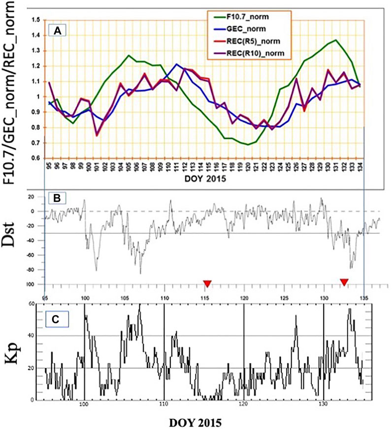
FIGURE 7. Solar-geophysical conditions during April−May 2015. Al Normalized values of: FI0.7—Solar electromagnetic radiation on the Wavelength 10.7 cm; GEC—Global ionospheric content, sum of all values in the IONEX table; REC (R5)—the Regional Ionospheric Content—within the 500 km radius circle; REC (RIO)—it is the Regional Ionospheric Content—Within the 1000 km radius circle; 8/ Dst equatorial geomagnetic index; Cl Planetary K-index (Kp* l 0, OMNI WEB Plus).

In Figure 7B we plotted the Dst (equatorial geomagnetic) index for the same period. One can see that we are dealing with a moderately disturbed period. From the Dst we can conclude that we have three moderate (with Dst ∼ −80 nT) geomagnetic storms: before the first earthquake and one started during the second earthquake. The other disturbances we can classify as small, not exceeding −30 nT (continuous line, bottom panel of Figure 8). The period is also characterized by the essential variations of F10.7 (min 100, max 155). Normalized F10.7 is shown as the green line in the upper panel of Figure 7. The F10.7 variations should be eliminated in the dTEC variations (defined in Eq.(3)) because they contribute to the running mean calculations. The first attempt to reveal the pre-earthquake variations having disturbed conditions is considering the difference between the Global TEC and Regional TEC (blue and red lines in Figure 7). As we see from the upper panel of Figure 7, the Global TEC follows the F10.7 with a delay of nearly 2 days (Afraimovich et al., 2008; Marchitelli, V et al., 2020). We exclude the difference in the vicinity of day 101 (April 10), which is a magnetic storm day. The most suspicious days are 111 (April 21) and 114 (April 24), when we may expect negative and positive anomalies. The differential GIM maps were computed for these days to check this supposition, which is presented in Figure 8. We see the strong negative (in crests) anomalies on April 21 and a powerful positive anomaly on April 24. The strength of the equatorial anomaly should change. Considering that the epicenter is inside the northern crest of EIA, we will express the strength of the TEC anomaly at the Northern crest to the TEC in the trough of EIA (Figure 9). We also calculate S - the strength of EIA on undisturbed days as a relation between the TEC value in the crest of anomaly and in trough between crests. On day 111 (April 21), the EIA completely disappears which gives its strength less than 1: S = 0.98. S- It is the strength of equatorial anomaly (relation between the TEC value in crest of anomaly and in trough between crests). On day 114 (April 24), the anomaly strength is 1.69, and on disturbed days before the earthquake—day 98 (April 07) and after the earthquake - days 117 (April 27) and 120 (April 30), the strength varied from 1.22 to 1.39.

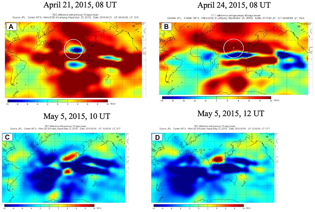
FIGURE 8. GIM GPSffEC spatial analysis. (A) Differential TEC map of April 21, 2015, (−4 days) 09UT and (B) April 24, 2015, 08UT (−1 day) (C) Differential TEC map of May 5, 2015, (−7 days) !OUT and (D) May 5, 2015, 12UT (−7 day).

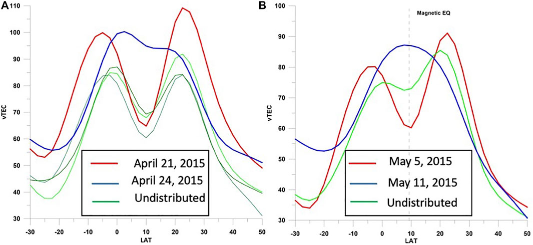
FIGURE 9. dTEC variations (defined in Eq. 3) for the lhaz GPS/GLONASS receiver (Figure 1) for April 6–May 15, 2015.

From the historical data of the ionosphere, monitoring has elaborated a conception of the precursor mask, which generalizes the pattern of ionosphere parameter variations (foF2 or GPS TEC) a few days before the earthquakes (Pulinets et al., 2007, 2018).

Where TEC—is the Total Electron Content in TECU, where TECU = 10¹⁶ el/m², TEC_m 15-days running average value of TEC. The precursor mask was developed based on the analysis of strong (M ≥ 6) earthquakes in Greece and Italy (Pulinets and Ouzounov, 2018; Davidenko and Pulinets, 2019). We used this approach to analyze the dTEC variations for the lhaz GPS receiver around the two Nepal earthquakes presented in Figure 10. The horizontal axis is the Day of Year 2015 of the mainshock designated by zero. Vertical axis—is the local time (LT), and VTEC deviation is color-coded in percentages relative to the 15-days mean. We can see that the positive anomaly appears near 8 PM and exists continuously up to 4 AM the next day. In the present figure, the anomalies appear 3 days before the mainshock. However, further analysis for other earthquakes revealed that such anomalies might appear up to 5 before the mainshock. We can see similar night-time positive deviations before both strong earthquakes lasting more than 1 day and repeating every day at the same local time. The only difference with the pattern presented in Figure 10 is that the favorable variations start at 6 PM and finish at 6 AM. It can relate to the different terminator times for Greece and Nepal (Zolotov, 2015).

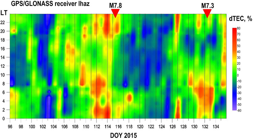
FIGURE 10. GIM GPSffEC spatial analysis. (A) Differential TEC map of April 21, 2015, (−4 days) 09UT and (B) April 24, 2015, 08UT (−1 day) (C) Differential TEC map of May 5, 2015, (−7 days) ! OUT and (D) May 5, 2015, 12UT (−7 day).

Very Low Frequency/Low Frequency (VLF/LF) Probing

One of the possible experimental techniques that can monitor the ionization’s perturbations within the lower ionosphere uses Very Low Frequency/Low Frequency (VLF/LF) probing. Waves in the VLF frequency range are trapped between the lower ionosphere and the Earth and are reflected by the D region at an altitude of ∼65 km during the daytime and ∼85 km during nighttime. The received signals contain information about the reflection height’s region and its variability (Barr et al., 2000). The propagation of sub ionospheric VLF/LF (15–50 kHz) signals from navigation or time service transmitters over distances of thousands of kilometers (with low attenuation ∼2–3 dB per Mm) enables remote sensing over large regions of the upper atmosphere in which ionospheric modifications lead to changes in the received amplitude and phase of the signals. The regular monitoring of many years at the Far East network, which operates in a highly seismic zones such as Japan and Kurile Islands, has established a statistical correlation between anomalies of the VLF/LF signal parameters in the nighttime and earthquakes with М ≥ 5.5. When observed, the possible time intervals of seismic-related phase and amplitude anomalies are about 1 week before an earthquake and 1 week after the event (Rozhnoi et al., 2004,2009,2015; Maekawa et al., 2006; Hayakawa et al., 2010, Biagi et al., 2011; Hayakawa 2015). Anomalies for such earthquakes were found in 20–25% of all cases. However, for strong earthquakes (M > 6.8), anomalies VLF/LF were observed in 60–70% of the earthquakes (Rozhnoi et al., 2013).

The VLF/LF receiving stations deployed both in Europe (Eastern Europe, Sheffield, Graz), the Far East (Kamchatka, Sakhalin, Kuril Islands), North America (Orange, CA) and Asia (Bishkek, Varanasi) are equipped with the UltraMSK receivers (http://ultramsk.com/). All the stations simultaneously receive the amplitude and phase of MSK (Minimum Shift Keying) modulated signals with fixed frequencies in a narrow band 50–100 Hz around the central frequency and adequate phase stability. The receivers can record signals with time resolutions ranging from 50 msec to 60 s. For our purpose, we use a sampling frequency of 20 s. The VLF/LF observation network is shown in Figure 11A, and the epicenters of earthquakes with M > 5 for the last 3 years. The analysis reported in this paper about earthquakes in Nepal in April-May 2015 is based on these data recorded by the VLF/LF stations in Bishkek (KGZ) and Varanasi (VAR).

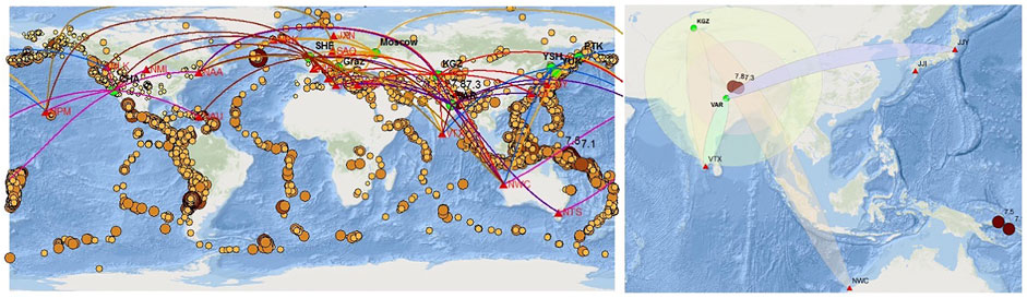
FIGURE 11. The VLF/LF network. Green circles show the positions of receiving stations. Red triangles show transmitters. The lines are propagations paths from the transmitters to receivers. Brown circles show the epicenters of earthquakes with M > 5.5 for the period 2013-2015. Bl A map of the wave paths under analysis together with the epicenters of earthquakes with M > 7 (solid brown circles) occurred in April-May 2015. KGZ stands for the station in Bishkek (Kirgizstan), VAR means the station in Varanasi (India), YSH is the station in Yuzhno-Sakhalinsk (Sakhalin Island). The areas of earthquake preparation where precursors can be found are shown by the yellow circle for the first larger earthquake on April 25 and the pink circle for the second earthquake on May 12, 2015. The ellipses are projections of the third Fresnel sensitivity zone on the Earth’s surface.

Figure 11B, shows the relative positions of our observing stations and transmitters VTX (17.0 kHz) in India, NWC (19.8 kHz) in Australia, and JJY (40 kHz) in Japan, together with the positions of the epicenters of earthquakes in April-May 2015 in the region under analysis. The areas of earthquake preparation where precursors can be found (Dobrovolsky et al., 1979) are shown by the pink circle for the first strong earthquake on April 25 and the yellow circle for the second earthquake on May 12, 2015. The station in Varanasi (VAR) began a regular reception in April; therefore, analysis for both stations were made from the beginning of April. Two wave paths—NWC-KGZ and JJY-VAR pass directly above the epicenter of the Nepal earthquake. The signal from the JJI transmitter received at the Varanasi (VAR) station also passes above the epicenter, but it was not used for the analysis because it is very noisy. Two sub-ionospheric paths (VTX-KGZ and VTX-VAR) are outside the epicenter but inside the earthquake preparation area. We used a residual signal of amplitude calculated as the difference between the actual signal and the monthly averaged signal for our analysis.

The last was calculated using the data from undisturbed days. Since VLF/LF signals are very stable during daytime and are unaffected by any force except X-rays emitted during solar flares, the analysis was made only for nighttime. The results of these analyses are shown in Figure 12A. For validation of the results, we analyzed the signals from the same NWC and JJY transmitters propagating far away from the seismic zone, the significant negative nighttime amplitude anomalies for the four paths crossing the area where the possible precursors of the earthquake can be found 4–5 days before the first earthquake while the signals in the “aseismic” paths vary insignificantly (Figure 12B). Then after several days, when the signals were quiet, the second series of anomalies can be seen. These anomalies continue after the earthquake during the period of aftershock activity.

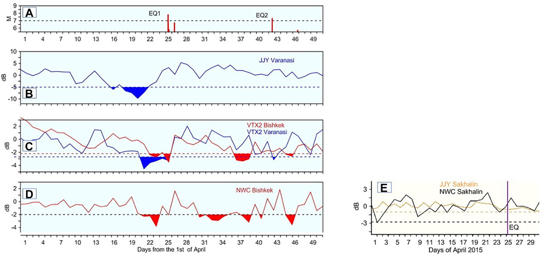
FIGURE 12. (A–D) The results of the VLF/LF analysis. The average residual amplitudes of the VLF/LF signals in the nighttime are shown (top to down) for vrx (17.0 kHz)transmitter recorded in Bishkek (red) and Varanasi (blue), NWC (19.8 kHz) transmitter recorded in Bishkek, JN (40 kHz) transmitter recorded in Varanasi. The bottom panel shows JJY (yellow) and NWC (black) transmitter signals recorded in Yuzhno-Sakhalinsk stations (control “aseismic” paths). The upper panel shows the occurrence time of the earthquakes. The color-filled zones indicate values exceeding the −2a (a is the standard deviation) lEvel, indicated by the horizontal dotted lines. Fl the controlled pa1hs NWS Sakhalin and JJY Sakhalin.

Discussion

A joint analysis of atmospheric and ionospheric parameters during the M7.8 earthquake in Nepal has demonstrated correlated variations of atmospheric anomalies implying their connection with the earthquake preparation processes. One of the possible explanations for this relationship is the Lithosphere- Atmosphere- Ionosphere Coupling mechanism (Pulinets and Boyarchuk, 2004; Pulinets and Ouzounov, 2011, Pulinets et al., 2018), which provides the physical links between the different geochemical, atmospheric and ionospheric variations and tectonic activity. This phenomenon’s primary process is the air ionization produced by increased radon emissions near active tectonic faults from the Earth’s crust. Through the air ionization, triggered by radon level increases, latent surface heat (SLHF) (Cervone et al., 2010) was rapidly developed OLR anomaly was formed at the top of the Atmosphere (TOA) (Ouzounov et al., 2007; 2018b; Xiong et al., 2010). The distinct difference in the thermal atmospheric field over the earthquake preparation area automatically creates vertical air convection, which leads to a pressure anomaly. This pressure anomaly is probably responsible for the stationary behavior of the front end of the jet stream over the vicinity of the future epicentral area (Ouzounov et al., 2011; Wu and Tikhonov, 2014). At this point, we see the transition from atmospheric to electromagnetic effects. It is well established that the ion cluster size is essential for the Atmospheric Boundary Layer (ABL) of the Earth’s atmosphere electric conductivity because of the different mobility of ions of different sizes (Hõrrak, 2001). The small and medium-size ions increase the ABL electric conductivity while the large ones if their concentration is high enough, will essentially decrease it. Considering the Global Electric Circuit conception (Pulinets and Davidenko, 2014), we can expect the increase of the vertical electric field gradient in the ABL conductivity drop, which will lead to the change of the ionosphere potential concerning the ground over the earthquake preparation area. As a high conductive media, the ionosphere will maintain its equipotentiality by modifying plasma concentration and temperature within the potential changes area. Due to high conductivity along the geomagnetic field lines, these irregularities will form the modified inner magnetosphere ducts. These ducts will trap the VLF emission inside the modified magnetospheric tube, creating an increased level of VLF noises within the modified tube.

Similarly, as for the Wenchuan earthquake, we observe the changes of the EIA strength and the latitudinal movements of the crests of EIA. During the adverse effect, the crest moved equatorward, and during the positive effect—poleward (Figure 9). We can conclude from this picture that this movement is at least 2.5°. As for many cases of other strong earthquakes analyzed, we observe the effect in the magnetically conjugated area of the southern hemisphere.

The maps and profiles of the equatorial anomaly were made using the Global Maps GIM TEC in the form of IONEX index. It is a product of IGS, which interpolates the data of all GPS receivers and inserts the model where we do not have receivers. The dTEC mask (Figure 10) was built using the data of Lhasa GPS receiver lhaz. Concerning the epicenter, the location of Lhaz is shown in Figure 1. The profiles of the equatorial anomaly were taken at the longitude of the epicenter. So, the IONEX and lhaz should not coincide exactly. There could be differences because of two factors: IONEX—interpolation map, and Lhaz are eastward from the epicenter, and ionospheric variations over there could be slightly different.

Regarding the external impact on the VLF/LF observations, the geomagnetic activities were during the middle of April 2020 (Figure 7; Table 1). A magnetic storm occurred on April, 17 to the 18th (UT) with Dst ∼ -79 nT. It was preceded by a proton burst and the relativistic electron fluxes recorded during the recovering stage of the storm. The storm itself does not influence signals propagation because the sudden commencement and main phase of the storm occurred when the analysis zone was sunlit. Another factor that can influence the behavior of the VLF/LF signals is atmospheric pressure fluctuations (Rozhnoi et al., 2014). According to data from the ground meteorological stations in Bishkek, Varanasi, no sharp changes in atmospheric pressure were recorded during the period when anomalies in the signals were detected. Unlike the first earthquake, the JJY signal was undisturbed before the second earthquake. It can relate to the signal’s frequency (its frequency is twice higher than the frequencies of other signals) or the direction of propagation. This signature is lost due to the signal in the ionosphere irregularities during propagation. Therefore in Figure 12B, only the −2σ (σ is the standard deviation) level is shown for all the paths. The decrease of the NWC signal in the middle of May in the “aseismic” path NWC-YSH most probably was caused by two very strong Typhoons-Noul (1,506) and Dolphin (1,507), which followed one after another and crossed the path at that time. So, considering the possible influence of other factors which can produce perturbations in VLF/LF signals and rejecting them, also using “aseismic” paths, we may conclude that impending earthquakes caused observed anomalies. The preparation/activation zone estimate for both the M7.8 Nepal earthquake on April 24, and the M7.3 on May 12, 2015 follow the Dobrovolsky/Bowman estimates (R = 10^0.43M/R = 10^0.44M), are areas with a radius of 2,259/2,703 km and 1,377/1,629 km accordingly. The soil Rn222 concentration profiles measured simultaneously at two nearby sites at Jadavpur University, Kolkata, India, was at 625 km distance from the epicenter of the April 24 M7.7 Nepal earthquake (Figure 3A). During March-May 2015, about 15 TRA anomalies were detected around the Nepali M7.3 epicentral areas (Figure 5) were inside the 2,259 km zone. With the VLF/LF analysis, the area of earthquake preparation where precursors can be found is shown in Figure 11B by the pink circle for the first earthquake of M7.8 on April 25 and the yellow circle for the M7.3 n May 12, 2015. Although the radon variations, TRA and VLF, were observed far from epicentral areas, the anomalies are inside the Dobrovolsky-Bowman earthquake preparation area estimate. The pre-seismic ionospheric effects for the 2015 Nepal earthquakes are typical for low latitude earthquakes involving the equatorial ionospheric anomaly (EIA). The positive and negative effects are reflected in the conjugated hemisphere due to the charged particles that are influenced by the geomagnetic field lines. These effects should not be considered for Dobrovolsky’s estimation. In addition, the equatorial effects are stretched along the longitude and exceed the Dobrovolsky size. Only the latitudinal size over the earthquake preparation area should be considered (Klimenko et al., 2011, Kuo et al., 2014 Pulinets et al., 2014, 2021). The complex study of the synergetic behaviors of earthquake precursors helped to understand the direction of the process development leading to the critical state of the geosystems (Sornette and Sammis, 1995; Yasuoka et al., 2006,2009; De Santis et al., 2010; Pulinets 2011). As part of this study, the temporal behavior of earthquake precursors has been revealed as a sequencing pattern (Pulinets and Ouzounov, 2018), and the accelerated trend in the pre-earthquake anomalies has been identified (De Santis et al., 2017; De Santis et al., 2020). Here we demonstrate the temporal trend of the pre-earthquake and their accelerating pattern as the earthquake approaches (Figure 13A, Figure 13B). The cumulative number of all revealed precursory anomalies shown on the temporal trend is indicated in Figure 13B with black circles and lines associated with M7.8 of April 25, 2015, and red circles and lines for M7.3 of May 12, 2015, as well. The time origin (t = 0) is the mainshock occurrence (blue line). With Red/Black, thick line curves show the fit exponential -growth with Equation f = 2.0813 + 9.7166 ^∗exp (0.1596 ^∗x) for the black curve (April 5, 2015, earthquake) and with Equation f = 2.5 + 292.8693 ^∗exp (4.5811 ^∗x) for the red curve (May 12 Earthquake) while Red/black is the straight line (thin lines). This graph confirms strong acceleration as the mainshocks approaching both earthquakes. We see different patterns in the temporal (13a) and cumulative exponential -growth graphs (13b, Black vs. Red) before the mainshock (April 25, 2,915) and that before the major aftershock (May 12, 2015). The increased aftershock activities contributed to the difference in preparation time (shorter for the major aftershock) and into the much steeper pattern.

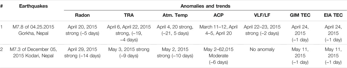
TABLE 1. Detection of joint anomalies for the M7.8 of 04.25.2015 Gorkha, Nepal and M7.3 of December 05, 2015 Kodari, Nepal.

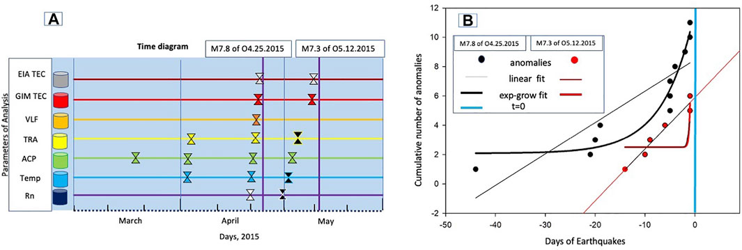
FIGURE 13. (A) Fime diagram of multiparameter precursors analysis plotted with data shown in Table 1. The list of analyzed parameters ( bottom-up): Rn (Radon gas); Temp (Meteorological Atmospheric temperature); ACP (Atmospheric chemical potential); TRA (Thermal Radiation Anomaly); VLF (Vert low Frequency); GIM TEC (Global Ionospheric Model, Total Electronic Contents); EIA TEC (Equatorial Ionospheric Anomaly, Total Electronic Contents); (B) Cumulative number of all revealed precursory anomalies shown on Panel 13a (indicated here as black circles and lines associated with M7.8 of April 25, 2015, and with red circles and lines for M7.3 of May 12, 2015, as well.); Time origin t = O is the mainshock occurrence (blue line). With Red/Black, thick line curves show the exp-grow fit while Red/black is the straight line (thin lines). This graph confirms strong acceleration as the mainshocks approach both earthquakes.

Conclusion

Our results show evidence that processes related to the Nepal earthquakes started at least in mid-March and were seen by satellite thermal observations (Figure 6; Table 1). On April 5, the atmospheric temperature had increased, which continued on April 23 with a thermal field build up on the top of the atmosphere (OLR) near the epicentral area (Figure 4). The ionosphere immediately reacts to these changes in the electric properties of the ground layer measured by GPS/TEC over the epicenter areas, which have been confirmed as a spatially localized increase in the dTEC on April 21 and 24 (Fig. 8,9,10,12). A similar scenario occurred for the M7.3 earthquake of May 12, 2015, with some delays in building the GPS/TEC, probably as a result of gas diffusion associated with the ground fracturing that occurred in the region during the first M7.8 earthquake. Ionospheric effects detected over the earthquake preparation zone, of the Nepal M7.8 earthquake, are very similar to those detected before the strong earthquakes in China (Wenchuan M7.9 earthquake on May 12, 2008, and Lushan M7.0 earthquake April 20, 2013) (Pulinets and Ouzounov, 2018). Configurations concerning the ionosphere morphology (position of the equatorial anomaly), is identical to the earthquakes that occurred in the Taiwanese region; because the Nepal earthquake’s epicenter vertical projection is on the outer edge of the northern crest of the equatorial anomaly. So, except for the analysis of effect per se, we confirmed the results of previous studies on the ionospheric effects of strong earthquakes (Pulinets and Ouzounov, 2018; Ouzounov et al., 2018a).

Multi-parameter data recording atmospheric and ionospheric conditions during the M7.8 and M7.3 earthquakes in Nepal; using OLR monitoring on the top of the atmosphere, GIM-GPS/TEC maps, vertical TEC of lhaz GPS/GLONASS receiver in the region. The VLF/LF over NWC-KGZ and JJY-VAR paths for the first strong earthquake, and atmospheric temperature from ground measurements show the presence of anomalies in the atmosphere and ionosphere occurring consistently over the region near the 2015 Nepal earthquake epicenter. These results show evolutionally patterns in the appearance of pre-earthquake transient effects in the atmosphere and ionosphere, with a short time-lag from hours up to a few days (Figure 13ab; Table 1), and scalable with a magnitude estimate at their unusually far distance from the epicenter. The spatial characteristics of pre-earthquake anomalies were associated with the larger area but always inside the preparation-activation region estimated by Dobrovolsky-Bowman.

Data Availability Statement

Not all the datasets presented in this article are readily available. Requests to access the datasets should be directed to ouzounov@chapman.edu.

Author Contributions

DO, SP and VF provided the concepts of the manuscript. DO organized and wrote the manuscript with the help of SP, VF, ARo, MS and PT. MK, BND, ARy provided critical feedback. All authors contributed to the submitted version of the article.

Conflict of Interest

The authors declare that the research was conducted in the absence of any commercial or financial relationships that could be construed as a potential conflict of interest.

Publisher’s Note

All claims expressed in this article are solely those of the authors and do not necessarily represent those of their affiliated organizations, or those of the publisher, the editors, and the reviewers. Any product that may be evaluated in this article, or claim that may be made by its manufacturer, is not guaranteed or endorsed by the publisher.

Acknowledgments

Thanks to ISC, USGS, EMSC for the seismic data. We thank NOAA/National Weather Service National Centers for Environmental Prediction Climate Prediction Center for providing OLR and surface temperature data. The IONEX data and RINEX data (for lhaz GPS/GLONASS receiver) in this study were acquired as part of NASA’s Earth Science Data Systems and archived and distributed by the Crustal Dynamics Data Information System (CDDIS). The Dst index was provided by Kyoto World Data Center for Geomagnetism (http://wdc.kugi.kyoto- u.ac.jp/dstdir/index.html). DO and SP also thank ISSI (Bern) for support of the team “Multi-instrument Space-Borne Observations and Validation of the Physical Model of the Lithosphere-Atmosphere-Ionosphere-Magnetosphere Coupling” who initiated the research on the 2015 Nepalian earthquakes. BD thanks Abhishek Srivastava for his help in handling the data. Authors are grateful to all reviewers for their valuable comments and suggestions.

References

Afraimovich, E. L., Astafyeva, E. I., Oinats, A. V., Yasukevich, Y. V., and Zhivetiev, I. V. (2008). A New conception to Track Solar Activity, Ann. Geophys. Global Electron Content, 26, 335–344.
Barr, R., Jones, D. L., and Rodger, C. J. (2000). ELF and VLF Radio Waves. J. Atmos. Solar-Terrestrial Phys. 62, 1689–1718. doi:10.1016/s1364-6826(00)00121-8
Biagi, P. F., Maggipinto, T., Righetti, F., Loiacono, D., Schiavulli, L., Ligonzo, T., et al. (2011).The European VLF/LF Radio Network to Search for Earthquake Precursors: Setting up and Natural/man-Made Disturbances, Nat. Hazards Earth Syst. Sci. 11, 333–341.doi:10.5194/nhess-11-333-2011
Bowman, D. D., Ouillon, G., Sammis, C. G., Sornette, A., and Sornette, D. (1998). An Observational Test of the Critical Earthquake Concept. J. Geophys. Res. 103 (24), 359372–359424. doi:10.1029/98jb00792
Boyarchuk, K. A., Karelin, A. V., and Nadolski, A. V. (2010). Statistical Analysis of the Chemical Potential Correction Value of the Water Vapor in Atmosphere on the Distance from Earthquake Epicenter. Issues electro Mech. 116, 39–46.
Cervone, G., Maekawa, S., Singh, R. P., Hayakawa, M., Kafatos, M., and Shvets, A. (2006). Surface Latent Heat Flux and Nighttime LF Anomalies Prior to the Mw=8.3 Tokachi-Oki Earthquake. Nat. Hazards Earth Syst. Sci. 6, 109–114. doi:10.5194/nhess-6-109-2006
Chen, S., Liu, M., Xing, L., Xu, W., Wang, W., Zhu, Y., et al. (2016). Gravity Increase before the 2015 Mw 7.8 Nepal Earthquake. Geophys. Res. Lett. 43. doi:10.1002/2015GL06659510.1002/2015gl066595
Contadakis, M. E. (2011). The European VLF/LF Radio Network to Search for Earthquake Precursors: Setting up and Natural/man-Made Disturbances. Nat. Hazards Earth Syst. Sci. 11, 333–341. doi:10.5194/nhess-11-333-2011
Davidenko, D. V., and Pulinets, S. A. (2019). Deterministic Variability of the Ionosphere on the Eve of Strong (M ≥ 6) Earthquakes in the Regions of Greece and Italy According to Long-Term Measurements Data. Geomagn. Aeron. 59 (4), 493–508. doi:10.1134/s001679321904008x
De Santis, A., Cianchini, G., Qamili, E., Frepoli, A., De Santis, A., Balasis, G., et al. (2010). Potential Earthquake Precursory Pattern from Space: The 2015 Nepal Event as Seen by Magnetic Swarm Satellites, Earth Planet. Sci. Lett., The 2009 L'Aquila (Central Italy) Seismic Sequence as a Chaotic Process, Tectonophysics, 496 44–52, 461, 19–126.
De Santis, A., Cianchini, G., Marchetti, D., Piscini, A., Sabbagh, D., Perrone, L., et al. (2020). A Multiparametric Approach to Study the Preparation Phase of the 2019 M7.1 Ridgecrest (California, United States) Earthquake. Front. Earth Sci., 8 doi:10.3389/feart.2020.540398
Deb, A., Gazi, M., and Barman, C. (2016). Anomalous Soil Radon Fluctuations - Signal of Earthquakes in Nepal and Eastern India Regions. J. Earth Syst. Sci. No. 8, 125. December, 1657–1665. doi:10.1007/s12040-016-0757-z
Dobrovolsky, I. P., Zubkov, S. I., Myachkin, V. I., and Miachkin, V. I. (1979). Estimation of the Size of Earthquake Preparation Zones. Pageoph 117, 1025–1044. doi:10.1007/bf00876083
Fu, C.-C., Lee, L.-C., Yang, T. F., Lin, C.-H., Chen, C.-H., Walia, V., et al. (2019). Gamma Ray and Radon Anomalies in Northern Taiwan as a Possible Preearthquake Indicator Around the Plate Boundary, Geofluids ID 4734513, 2019, 1–14. doi:10.1155/2019/4734513
Fu, C.-C., Wang, P.-K., Lee, L.-C., Lin, C.-H., Chang, W.-Y., Giuliani, G., et al. (2015). Temporal Variation of Gamma Rays as a Possible Precursor of Earthquake in the Longitudinal Valley of Eastern Taiwan. J. Asian Earth Sci. 114, 362–372. doi:10.1016/j.jseaes.2015.04.035
Giuliani, G., Attanasio, A., and Fioravanti, G. (2013). Gamma Detectors for Continuous Monitoring of Radon. J. Int. Environ. Appl. Sci. 8 (4), 541–550.
Gruber, A., and Krueger, A. F. (1984). The Status of the NOAA Outgoing Longwave Radiation Data Set. Bull. Amer. Meteorol. Soc. 65, 958–962. doi:10.1175/1520-0477(1984)065<0958:tsotno>2.0.co;2
Harris, G. (2015). Everest Climbers Are Killed as Nepal Quake Sets off Avalanche. New York: NY Times.
Hayakawa, M. (2013). Earthquake Prediction Studies: Seismo Electromagnetics. Tokyo, Japan: TERRAPUB, 168.
Hayakawa, M., Kasahara, Y., Nakamura, T., Muto, F., Horie, T., Maekawa, S., et al. (2010). A Statistical Study on the Correlation between Lower Ionospheric Perturbations as Seen by Subionospheric VLF/LF Propagation and Earthquakes. J. Geophys. Res. 115, a–n. doi:10.1029/2009JA015143
Hõrrak, U. (2001). “Contribution of Air Ion Mobility Classes to Air Conductivity,”Dissertationes Geophysicales Universitatis Tartuensis. in Air Ion Mobility Spectrum at a Rural Area (Tartu, Estonia: Tartu University), 15, 81.
Karastathis, V. K., Eleftheriou, G., Tselentis, A., Tsinganos, K., Kafatos, M., Ouzounov, D., et al. (2019). Real-time Monitoring of Soil Radon Concentration at Seismically Active Areas in Greece in -18, 27th IUGG Assembly (Montreal Canada.
Klimenko, M. V., Klimenko, V. V., Zakharenkova, I. E., Pulinets, S. A., Zhao, B., and Tsidilina, M. N. (2011). Formation Mechanism of Great Positive TEC Disturbances Prior to Wenchuan Earthquake on May 12, 2008. Adv. Space Res. 48, 488–499. doi:10.1016/j.asr.2011.03.040
Kolvankar, V., More, S., and Thakur, N. (2010). Earth Tides and Earthquakes. New Concepts Glob. Tectonics Newsl. 57, 54–84.
Kon, S., Nishihashi, M., and Hattori, K. (2010). Ionospheric Anomalies Possibly Associated with M>=6.0 Earthquakes in the Japan Area during 1998-2010: Case Studies and Statistical Study. J. Asian Earth Sci. 41 (4‐5), 410–420. doi:10.1016/j.jseases.2010.10.005
Kuo, C. L., Lee, L. C., and Huba, J. D. (2014). An Improved Coupling Model for the Lithosphere-Atmosphere-Ionosphere System. J. Geophys. Res. Space Phys. 119, 3189–3205. doi:10.1002/2013ja019392
Li, W., Guo, J., Yue, J., Yang, Y., Li, Z., and Lu, D. (2016). Contrastive Research of Ionospheric Precursor Anomalies between Calbuco Volcanic Eruption on April 23 and Nepal Earthquake on April 25, 2015. Adv. Space Res. 57 (10), 2141–2153. doi:10.1016/j.asr.2016.02.014
Liu, J. Y., Chuo, Y. J., Shan, S. J., Tsai, Y. B., Chen, Y. I., Pulinets, S. A., et al. (2004). Pre-earthquake Ionospheric Anomalies Registered by Continuous GPS TEC Measurements. Ann. Geophys. 22, 1585–1593. doi:10.5194/angeo-22-1585-2004
Maekawa, S., Horie, T., Yamauchi, T., Sawaya, T., Ishikawa, M., Hayakawa, M., et al. (2006). A Statistical Study on the Effect of Earthquakes on the Ionosphere, Based on the Subionospheric LF Propagation Data in Japan. Ann. Geophys. 24, 2219–2225. doi:10.5194/angeo-24-2219-2006
Marchitelli, V., Harabaglia, P., TroiseDe Natale, C. G., and De Natale, G. (2020). On the Correlation between Solar Activity and Large Earthquakes Worldwide. Sci. Rep. 10, 11495. doi:10.1038/s41598-020-67860-3
Maurya, A. K., Venkatesham, K., Tiwari, P., Vijaykumar, K., Singh, R., Singh, A. K., et al. (20162016). The 25 April 2015 Nepal Earthquake: Investigation of Precursor in VLF Subionospheric Signal. J. Geophys. Res. Space Phys. 121. doi:10.1002/2016JA022721
Mehta, A., and Susskind, J. (1999). Outgoing Longwave Radiation from the TOVS Pathfinder Path A Data Set. J. Geophys. Res. 104, NO. D10, 12193–12212. doi:10.1029/1999jd900059
Němec, F., Santolík, O., Parrot, M., and Berthelier, J. J. (2008). Spacecraft Observations of Electromagnetic Perturbations Connected with Seismic Activity. Geophys. Res. Lett. 35, L05109. doi:10.1029/2007GL032517
Ohring, G., and Gruber, A. (1982). Satellite Radiation Observations and Climate Theory. Adv. Geophys. 25, 237–304.
Oikonomou, C., Haralambous, H., and Muslim, B. (2016). Investigation of Ionospheric TEC Precursors Related to the M7.8 Nepal and M8.3 Chile Earthquakes in 2015 Based on Spectral and Statistical Analysis. Nat. Hazards 83, 97–116. doi:10.1007/s11069-016-2409-7
Ouzounov, D., Bryant, N., Logan, T., Pulinets, S., and Taylor, P. (2006). Satellite thermal IR Phenomena Associated with Some of the Major Earthquakes in 1999-2003. Phys. Chem. Earth, Parts A/B/C 31, 154–163. doi:10.1016/j.pce.2006.02.036
Ouzounov, D., Liu, D., Chunli, K., Cervone, G., Kafatos, M., and Taylor, P. (2007). Outgoing Long Wave Radiation Variability from IR Satellite Data Prior to Major Earthquakes. Tectonophysics 431, 211–220. doi:10.1016/j.tecto.2006.05.042
Ouzounov, D., Pulinets, S., and Davidenko, D. (2015). Revealing Pre- Earthquake Signatures in Atmosphere and Ionosphere Associated with 2015 M7.8 and M7.3 Events in NepalPreliminary Results. Available at: https://arxiv.org/abs/1508.01805.
Ouzounov, D., Pulinets, S., Hattori, K., and Taylor Ed’s, P. (2018a). Pre-Earthquake Processes: A Multi-Disciplinary Approach to Earthquake Prediction Studies. American Geophysical UnionJohn Wiley & Sons, Inc., 385. Available at: https://agupubs.onlinelibrary.wiley.com/doi/book/10.1002/9781119156949.
Ouzounov, D., Pulinets, S., Kafatos, M. C., Taylor, P., Ouzounov, D., Pulinets, S., et al. (2018b). “Thermal Radiation Anomalies Associated with Major Earthquakes,” in The Book “Pre-earthquake Processes: A Multidisciplinary Approach to Earthquake Prediction Studies”, Geophysical Monograph 234. Multiparameter Assessment of Pre‐Earthquake Atmospheric Signals; in the Book “Pre-earthquake Processes: A Multidisciplinary Approach to Earthquake Prediction Studies”, Geophysical Monograph 234. Editors D. Ouzounov, S. Pulinets, K. Hattori, and P. Taylor (AGU & WileyAGU & Wiley), 259339–274357. doi:10.1002/9781119156949.ch15
Ouzounov, D., Pulinets, S., Romanov, A., Romanov, A., Tsybulya, K., Davidenko, D., et al. (2011c). Atmosphere-ionosphere Response to the M9 Tohoku Earthquake Revealed by Multi-Instrument Space-Borne and Ground Observations: Preliminary Results. Earthq Sci. 24, 557–564. doi:10.1007/s11589-011-0817-z
Parrot, M. (2009).Anomalous Seismic Phenomena: View from Space, in The Book: Electromagnetic Phenomena Associated with Earthquakes (Ed. by M. Hayakawa), Transworld Research Network, 205–233.
Prakash, R., Singh, R. K., and Srivastava, H. N. (2015). Outgoing Long Wave Radiation (OLR) from Kalpana Satellite Prior to Nepal Earthquake of April 25, 2015 IJRET: Int. J. Res. Eng. Tech. eISSN 2319-1163, 2321–7308
Pulinets, O. D. S., Hattori, K. M., and Kafatos, P. Taylor. (2011b). “Atmospheric Signals Associated with Major Earthquakes. A Multi-Sensor Approach,” in The Book Frontier of Earthquake Short-Term Prediction Study. Editor M. Hayakawa (Springer- Nature: Japan), 510–531.
Pulinets, S., Ouzounov, D., Karelin, A., and Davidenko, D. (2018). “Lithosphere–Atmosphere–Ionosphere–Magnetosphere Coupling—A Concept for Pre‐Earthquake Signals Generation,” in The Book “Pre-earthquake Processes: A Multidisciplinary Approach to Earthquake Prediction Studies”, Geophysical Monograph 234. Editors D. Ouzounov, S. Pulinets, K. Hattori, and P. Taylor (Bristol, UK: AGU & Wiley), 79–99.
Pulinets, S. A., and Boyarchuk, K. A. (2004). Ionospheric Precursors of Earthquakes. Berlin, Heidelberg, New York: Springer, 315.
Pulinets, S. A., Kotsarenko, A. N., Ciraolo, L., and Pulinets, I. A. (2007). Special Case of Ionospheric Day-To-Day Variability Associated with Earthquake Preparation. Adv. Space Res. 39, 970–977. doi:10.1016/j.asr.2006.04.032
Pulinets, S. A., Ouzounov, D., Karelin, A. V., Boyarchuk, K. A., and Pokhmelnykh, L. A. (2006). The Physical Nature of Thermal Anomalies Observed before Strong Earthquakes. Phys. Chem. Earth, Parts A/B/C 31, 143–153. doi:10.1016/j.pce.2006.02.042
Pulinets, S., and Davidenko, D. (2014). Ionospheric Precursors of Earthquakes and Global Electric Circuit. Adv. Space Res. 53 (5), 709–723. doi:10.1016/j.asr.2013.12.035
Pulinets, S., Ouzounov, D., Davidenko, D., and Budnikov, P. (2020). Principles of Organizing Earthquake Forecasting Based on Multiparameter Sensor-WEB Monitoring Data. E3s Web Conf. 196, 03004. doi:10.1051/e3sconf/202019603004
Pulinets, S., and Ouzounov, D. (2011). Lithosphere–atmosphere–ionosphere Coupling (LAIC) Model–A Unified Concept for Earthquake Precursors Validation. J. Asian Earth Sci. 41 (4), 371–3822. doi:10.1016/j.jseaes.2010.03.005
Pulinets, S., and Ouzounov, D. (2018). The Possibility of Earthquake Forecasting: Learning from Nature. Bristol, UK: Institute of Physics Books, IOP Publishing, 168pp.
Pulinets, S. (2011). The Synergy of Earthquake Precursors. Earthq Sci. 24, 535–548. doi:10.1007/s11589-011-0815-1
Pulinets, S., Tsidilina, M., Ouzounov, D., and Davidenko, D. (2021). From Hector Mine M7.1 to Ridgecrest M7.1 Earthquake. A Look from a 20-Year Perspective. Atmosphere 12, 262. doi:10.3390/atmos12020262
Qi, Y., Wu, L., Ding, Y., and Mao, W. (2020). Microwave Brightness Temperature Anomalies Associated with the 2015 Mw 7.8 Gorkha and Mw 7.3 Dolakha Earthquakes in Nepal. IEEE Trans. Geosci. Remote Sensing 2020 (99), 1–11. doi:10.1109/TGRS.2020.3036079
Rozhnoi, A., Solovieva, M., Levin, B., Hayakawa, M., and Fedun, V. (2014). Meteorological Effects in the Lower Ionosphere as Based on VLF/LF Signal Observations. Nat. Hazards Earth Syst. Sci. 14, 2671–2679. doi:10.5194/nhess-14-2671-2014
Rozhnoi, A., Solovieva, M., Molchanov, O., Schwingenschuh, K., Boudjada, M., Biagi, P. F., et al. (2009). Anomalies in VLF Radio Signals Prior the Abruzzo Earthquake (M=6.3) on 6 April 2009. Nat. Hazards Earth Syst. Sci. 9, 1727–1732. doi:10.5194/nhess-9-1727-2009
Rozhnoi, A., Solovieva, M., Parrot, M., Hayakawa, M., Biagi, P.-F., Schwingenschuh, K., et al. (2015). VLF/LF Signal Studies of the Ionospheric Response to strong Seismic Activity in the Far Eastern Region Combining the DEMETER and Ground-Based Observations. Phys. Chem. Earth, Parts A/B/C 85-86, 141–149. doi:10.1016/j.pce.2015.02.005
Rozhnoi, A., Solovieva, M. S., and Hayakawa, M. (2013). “VLF/LF Signals Method for Searching of Electromagnetic Earthquake Precursors Earthquake Prediction Studies,” in Book Seismo Electromagnetics, TERRAPUB (Tokyo: Masashi Hayakawa), 31–48.
Rozhnoi, A., Solovieva, M. S., Molchanov, O. A., and Hayakawa, M. (2004). Middle Latitude LF (40 kHz) Phase Variations Associated with Earthquakes for Quiet and Disturbed Geomagnetic Conditions. Phys. Chem. Earth, Parts A/B/C 29, 589–598. doi:10.1016/j.pce.2003.08.061
Scholz, C. H., Sykes, L. R., and Aggarwal, Y. P. (1973). Earthquake Prediction: A Physical Basis. Science 181, 4102803–4102810. doi:10.1126/science.181.4102.803
Shah, M., and Jin, S. (2016), Pre-seismic thermal Anomalies of the 2015 Mw = 7:8 Gorkha (Nepal) Earthquake from MODIS Surface Temperature. Progress in Electromagnetic Research Symposium. Shanghai, China: PIERS), 4755–4758. doi:10.1109/PIERS.2016.7735743
Sornette, D., and Sammis, C. G. (1995). Complex Critical Exponents from Renormalization Group Theory of Earthquakes: Implications for Earthquake Predictions. J. Phys. France 5, 607–619. doi:10.1051/jp1:1995154
Tramutoli, V., Aliano, C., Corrado, R., Filizzola, C., Genzano, N., Lisi, M., et al. (2013). On the Possible Origin of Thermal Infrared Radiation (TIR) Anomalies in Earthquake-Prone Areas Observed Using Robust Satellite Techniques (RST). Chem. Geology. 339, 157–168. doi:10.1016/j.chemgeo.2012.10.042
Tramutoli, V., Cuomo, V., Filizzola, C., Pergola, N., and Pietrapertosa, C. (2005). Assessing the Potential of thermal Infrared Satellite Surveys for Monitoring Seismically Active Areas: The Case of Kocaeli (İzmit) Earthquake, August 17, 1999. Remote Sensing Environ. 96, 409–426. doi:10.1016/j.rse.2005.04.006
Tronin, A. A., Hayakawa, M., and Molchanov, O. A. (2002). Thermal IR Satellite Data Application for Earthquake Research in Japan and China. J. Geodynamics 33, 519–534. doi:10.1016/s0264-3707(02)00013-3
Wu, H.-C., and Tikhonov, I. N. (2014). Jet Streams Anomalies as Possible Short-Term Precursors of Earthquakes with M>6.0. Res. Geophys. 4, 4939. doi:10.4081/rg.2014.4939
Xiong, P., Shen, X. H., Bi, Y. X., Kang, C. L., Chen, L. Z., Jing, F., et al. (2010). Study of Outgoing Longwave Radiation Anomalies Associated with Haiti Earthquake. Nat. Hazards Earth Syst. Sci. 10, 2169–2178. doi:10.5194/nhess-10-2169-2010
Yasuoka, Y., Igarashi, G., Ishikawa, T., Tokonami, S., and Shinogi, M. (2006). Evidence of Precursor Phenomena in the Kobe Earthquake Obtained from Atmospheric Radon Concentration. Appl. Geochem. 21, 1064–1072. doi:10.1016/j.apgeochem.2006.02.019072
Yasuoka, Y., Kawada, Y., Nagahama, H., Omori, Y., Ishikawa, T., Tokonami, S., et al. (2009). Preseismic Changes in Atmospheric Radon Concentration and Crustal Strain. Phys. Chem. Earth, Parts A/B/C 34, 431–434. doi:10.1016/j.pce.2008.06.005
Zhou, Y., Yang, J., Zhu, F., Su, F., HuZhai, L. W., and Zhai, W. (2017). Ionospheric Disturbances Associated with the 2015 M7.8 Nepal earthquake7.8 Nepal Earthquake. Geodesy and Geodynamics 8 (4), 221–228. doi:10.1016/j.geog.2017.04.004
Zolotov, O. V. (2015). Earthquake Effects in Variations of the Total Electron Content. Murmansk, Russia: Murmansk Arctic State University, 146.
Keywords: Nepal Earthquake, Natural hazards, precursors, thermal anomaly, ionospheric effects, GPS/TEC, VLF, LAIC
Citation: Ouzounov D, Pulinets S, Davidenko D, Rozhnoi A, Solovieva M, Fedun V, Dwivedi BN, Rybin A, Kafatos M and Taylor P (2021) Transient Effects in Atmosphere and Ionosphere Preceding the 2015 M7.8 and M7.3 Gorkha–Nepal Earthquakes. Front. Earth Sci. 9:757358. doi: 10.3389/feart.2021.757358
Received: 12 August 2021; Accepted: 29 October 2021;
Published: 23 November 2021.
Edited by:
Dmitry Efremenko, Helmholtz Association of German Research Centers (HZ), GermanyReviewed by:
Angelo De Santis, Istituto Nazionale di Geofisica e Vulcanologia (INGV), ItalyDedalo Marchetti, Jilin University, China
Lixin Wu, Central South University, China
Oleg Zolotov, Murmansk Arctic State University, Russia
Copyright © 2021 Ouzounov, Pulinets, Davidenko, Rozhnoi, Solovieva, Fedun, Dwivedi, Rybin, Kafatos and Taylor. This is an open-access article distributed under the terms of the Creative Commons Attribution License (CC BY). The use, distribution or reproduction in other forums is permitted, provided the original author(s) and the copyright owner(s) are credited and that the original publication in this journal is cited, in accordance with accepted academic practice. No use, distribution or reproduction is permitted which does not comply with these terms.
*Correspondence: Dimitar Ouzounov, ouzounov@chapman.edu