
Evaluation of the Continuous Monitoring of Land Disturbance Algorithm for Large-Scale Mangrove Classification


1
Department of Geography and Earth Sciences, Aberystwyth University, Aberystwyth SY23 3DB, UK
2
Plymouth Marine Laboratory, Prospect Place, Plymouth PL1 3DH, UK
3
Environment Systems Ltd., 9 Cefn Llan Science Park, Aberystwyth SY23 3AH, UK
*
Author to whom correspondence should be addressed.
Remote Sens. 2021, 13(19), 3978; https://doi.org/10.3390/rs13193978
Submission received: 23 August 2021
/
Revised: 13 September 2021
/
Accepted: 23 September 2021
/
Published: 5 October 2021
(This article belongs to the Section Forest Remote Sensing)
Abstract
:Mangrove forests are of high biological, economic, and ecological importance globally. Growing within the intertidal zone, they are particularly vulnerable to the effects of climate change in addition to being threatened on local scales by over-exploitation and aquaculture expansion. Long-term monitoring of global mangrove populations is therefore highly important to understanding the impact of these threats. However, data availability from satellites is often limited due to cloud cover. This problem can be mitigated using a season-trend modelling approach such as Continuous Monitoring of Land Disturbance (COLD). COLD operates by using every available observation on a pixel-wise basis, removing the need for whole cloud free images. The approach can be used to better classify land cover by taking into account the underlying seasonal variability, and can also be used to extrapolate between data points to obtain more accurate long term trends. To demonstrate the utility of COLD for global mangrove monitoring, we applied it to five study sites chosen to represent a range of mangrove species, forest types, and quantities of available data. The COLD classifier was trained on the Global Mangrove Watch 2010 dataset and applied to 30 years of Landsat data for each site. By increasing the period between model updates, COLD was successfully applied to all five sites (2253 scenes) in less than four days. The method achieved an overall accuracy of 92% with a User’s accuracy of 77% and a Dice score of 0.84 for the mangrove class. The lowest User’s accuracy was for North Kalimantan (49.9%) due to confusion with mangrove palms. However, the method performed extremely well for the Niger Delta from the 2000s onwards (93.6%) despite the absence of any Landsat 5 data. Observation of trends in mangrove extent over time suggests that the method was able to accurately capture changes in extent caused by the 2014/15 mangrove die-back event in the Gulf of Carpentaria and highlighted a net loss of mangroves in the Matang Forest Reserve over the last two decades, despite ongoing management. COLD is therefore a promising methodology for global, long-term monitoring of mangrove extent and trends.
1. Introduction
Mangrove forests exist in tropical and sub-tropical regions across the globe, covering a total area of nearly 140,000 km [1,2]. Growing within the intertidal zone, mangroves occupy a narrow ecological niche and are well adapted to saline environments and harsh coastal conditions [1,3]. Mangrove forests are of high biological, economic, and ecological importance globally [1,3], being a source of food, timber, and traditional medicines in addition to aiding in shoreline stabilisation by trapping sediment and nutrients and protecting coasts from the effects of cyclones and tsunamis [4,5,6]. Mangrove forests are also important carbon sinks [7], containing on average 1023 Mg per hectare and representing as much as 10% of carbon emissions from deforestation while only accounting for 0.7% of tropical forest globally [8].
Despite their importance, mangrove ecosystems across the globe are under threat [1,3,9,10,11]. While mangroves are tolerant of environmental change brought by tidal inundation, seasonal rainfall, and storms [11,12], their ecosystems are vulnerable to the effects of climate change and human activity [9]. As sea levels rise, inland areas become more frequently inundated with seawater, causing forests to retreat from the shoreline as their tolerance is exceeded [10,11]. On local scales, conversion to aquaculture (e.g., shrimp farming) is a major threat [3,13], accounting for around 38% of mangrove forest loss worldwide [13]. In addition, over-exploitation for fuel and timber has resulted in the degradation of a quarter of the world’s mangrove forest [13] and mangroves continue to be threatened by increasing human populations, industrialisation, urbanisation, and exploitation of natural resources such as oil [3,13,14,15]. A total of 16% of mangrove species are estimated to be at increased risk of extinction [13]. These pressures, combined with an increasing likelihood of extreme weather events such as cyclones and tsunamis [16], make the assessment and monitoring of mangrove forests a major concern.
This requirement for monitoring is difficult to meet even on regional scales due to the size and diversity of mangrove forests. Mangrove ecosystems are often highly dynamic, with constant erosion and deposition of sediment causing mangrove expansion and retreat, sometimes on very rapid timescales [17]. To accurately monitor these regions requires data collection from the whole forest to obtain a simultaneous snapshot of the entire area. However, for many mangrove forests, field studies are time consuming and expensive due to the size of the area covered and difficulty of access [18,19]. Remote sensing offers a solution to this problem, with satellites such as the Landsat and Sentinel missions capturing medium-scale spatial resolution data over large tracts of land on weekly timescales. These data have been widely utilised over the last few decades for forest monitoring [20,21,22] and for mangrove monitoring specifically [23,24,25]. However, while the need for global mangrove monitoring and assessment has long been identified [23,25], global assessments of mangrove extent and condition remain sparse and are often spatially inconsistent [24].
Several attempts have been made to rectify this knowledge gap. Giri et al. used Landsat data to estimate global mangrove extent for the year 2000 [1], but the study lacked an effective global validation method and did not report classification accuracy. Thomas et al. built on this work to compare mangrove extent between 1996 and 2010 using Japanese Earth Resources Satellite (JERS-1) and Advanced Land Observing Satellite Phased Array-type L-band Synthetic Aperture Radar (ALOS-PALSAR) data [26]. Validation was carried out using Landsat data with the study achieving high accuracy. Based mainly on Landsat and ALOS-PALSAR data, the Global Mangrove Watch (GMW) is a collaborative effort and represents the most recent and accurate map of global mangrove extent [2]. In addition to a baseline map for 2010, the GMW has also produced estimates of mangrove change from the mid-1990’s onwards. The issues with these efforts are that they either only provide an extent for a single year [1] or provide year-to-year comparisons based on composite imagery, often with large gaps in the change record [2,26]. While overall accuracy for the GMW is high (94%), the GMW methodology is time consuming, relying on multiple data sets and multiple classification steps in addition to manual quality assurance [2].
Recent developments in the field of land cover monitoring have lead to movement away from year-to-year comparisons of imagery and towards methods which make use of all available observations [27]. The rise of dense time series approaches such as Breaks for Additive and Seasonal Trend (BFAST) [28], Exponentially Weighted Moving Average Change Detection (EWMACD) [29], and Continuous Change Detection and Classification (CCDC) [30] provides a potential solution to the problem of global, long-term monitoring of mangrove extent. These methods use a season-trend modelling approach which captures the seasonal dynamics of land cover while also accounting for changes in condition. Applied on a per-pixel basis, such methodologies reduce reliance on individual observations and on individual cloud-free images, instead relying on the data record for each individual pixel through time. This is especially an advantage for mangrove monitoring, given that mangroves typically grow in tropical and sub-tropical regions with high cloud cover [3].
An additional advantage of these methods is that they allow for the extrapolation of existing data sets. For example, CCDC works by classifying each season-trend model rather than each point in time. A model might cover any time span from a year to multiple decades. By taking an existing, accurate data set such as the GMW, a classifier can be trained based on the models covering the period of that data set. This classifier can then be used to classify all models across time and space, allowing for the generation of yearly and sub-yearly extent estimates without the need for repeating the original, time consuming methodology. This process therefore allows for highly accurate but time-limited data sets such as the GMW to easily be extrapolated through time. In a previous study, we demonstrated that the CCDC method trained using GMW data could produce highly accurate maps of mangrove extent over the Sundarbans mangrove forest, in addition to tracking changes in mangrove condition over 30 years [31].
In this study, we apply the Continuous Monitoring of Land Disturbance algorithm (COLD) to each of five study sites to produce output detailing when class changes (i.e., mangrove to water) occurred. The COLD algorithm [32] is an update on the previous CCDC algorithm [30] for monitoring class changes in multi-band Landsat time series. The advantage of COLD for tropical forest monitoring is that it operates on a per-pixel basis, taking into account every available observation in the time series and fitting a model to the underlying land cover signal. This removes the requirement for finding cloud-free images for comparison and, since observations from different years are unlikely to fall on the same Day of Year (DOY), the effect of missing data is mitigated when applied to long time series. CCDC has previously been demonstrated to be an effective method for long-term mangrove classification and monitoring [31].
The aim of this study is to demonstrate the applicability of COLD for global mangrove monitoring using the Landsat data archive. Such an approach has potential to produce high quality estimates of mangrove extent which take into account intra-year fluctuations in addition to providing information on long term loss, gain, and trends. Five study sites are selected from across the globe to represent a range of mangrove species and forest types, with a variety of land cover change drivers. These sites also vary widely in the quantity of available data. Yearly mangrove extent for each site is calculated and tracked over time, with comparison to the GMW and other mangrove extent studies. Validation is performed through expert manual interpretation of Landsat and Google Earth imagery. The efficiency and feasibility of the method applied in Awty-Carroll et al. [31] for global mangrove monitoring is demonstrated and discussed.
2. Materials and Methods
2.1. Study Areas
2.2. Niger Delta, Nigeria
Draining into the Gulf of Guinea on the coast of southern Nigeria, the Niger River delta is one of the world’s largest wetlands covering an area of approximately 70,000 km [14]. It contains Africa’s largest contiguous mangrove forest [12] and the third largest mangrove forest globally [48]. The dominant mangrove species in the area are Rhizophora racemosa, R. mangle, and R. harrisonii with Avicennia germinans and Laguncularia racemosa also present [34,35]. The Niger Delta is also Africa’s largest river delta and is home to around 20% of Nigeria’s population [48]. The area used in this study is located from to N and to E (Figure 2A), covered by Worldwide Reference System-2 (WRS-2) Path 189 Row 57 (Table 1).
The region experiences very high annual rainfall (Table 1), with two peaks in July and September, a short dry season in August, and a longer dry season from October to March [14]. The delta is rich in biological resources, with mangroves being used for fuel, wood, fish trapping, local craft and construction. However, there is concern that local populations are over-dependent on the mangrove forest, especially for fuel wood [14]. The Niger Delta also has large oil and gas deposits which have been heavily exploited for decades [48], contributing substantially to mangrove forest loss [14]. The expansion of the oil industry typically involves the creation of canals for exploration and access, causing contamination of freshwater systems with seawater and destroying local ecosystems [49]. In addition, since the 1970’s there have been multiple unrecovered oil spills [49], causing widespread damage to the mangrove forest [48]. Estimates suggest that between 9 and 13 million barrels of oil have been spilled in the Niger Delta since 1958 [50].
Despite the ecological significance of the Niger Delta, mangroves and the potential negative effects of oil and timber exploitation, the region is generally under-studied. While several studies have been carried out which utilise remote sensing [12,33,48,49], these have been limited to comparisons between single images, offering change analysis on a five to ten year scale. This limitation can be attributed to the high cloud cover in the region, which makes it difficult to find suitable images for comparison (Figure 3).
2.3. Area around Cayenne, French Guiana
At 1500 km, the coast of north eastern South America is the longest muddy coast in the world [37]. Stretching from the mouth of the Orinoco to the mouth of the Amazon river, the coastal geology in this region is dominated by the large-scale deposition of sediment from the Amazon [17,37]. This particulate discharge forms mud banks up 60 km long and 30 km wide, which migrate along the coast of French Guiana towards the Orinoco at a rate of up to 3 km per year [51]. This migration creates a particularly unstable and dynamic coastline, with rapid and constant erosion and accretion [17,37]. The climate is hot and humid year round, with high levels of rainfall.
Mangroves cover an area of approximately 700 km across the coastline of French Guiana [36]. However, there is a complex relationship between mud bank migration and mangrove advance and retreat along the shoreline which makes mangrove dynamics in this region difficult to predict in the long term [51]. Typically, the presence of mud banks leads to the formation of large intertidal mud flats which are colonized by mangroves before the onward migration of the mud banks causes a loss of protection followed by massive erosion and mangrove retreat [17,51]. As a result, mangroves along the French Guianese coastline can be characterized into four development stages which exist roughly parallel to the coastline, from early growth and establishment to declining and dead mangrove forest [38]. Avicennia germinans is the dominant species, forming pioneer stands alongside Laguncularia racemosa in addition to making up the majority of the adult-age mangrove stands, with stands increasing in age with distance from the sea [36,38]. Other species present include Laguncularia racemosa and Rhizophora mangle, the former being a pioneer species which grows close to the shoreline, whereas the latter is less salt-tolerant and grows further inland [36].
The area used in this study is located from to N and to W (Figure 2B), covered by WRS-2 Path 227 Row 57 (Table 1). While studies have been carried out in this region which utilise satellite data [36,51,52], there are no current studies which make full use of the Landsat archive to monitor mangrove extent over time.
2.4. North Kalimantan, Borneo Island
An area rich in biodiversity, Borneo is the third largest island in the world [53]. Kalimantan is the Indonesian part of the island and represents approximately three-quarters of its area, with the remaining quarter being split between Malaysia and Brunai [54]. The climate is characterised by frequent rainfall and high temperatures year round [54]. In addition to mangroves, Borneo’s forests include dipterocarp, freshwater, peat, swamp, and heath forests, as well as nipah or mangrove palms, which grow in coastal regions alongside mangroves [53]. Specific information on mangrove species composition in North Kalimantan is difficult to find, but the area is likely dominated by Avicennia sp. amd Sonneratia sp. [41] with Rhizophora apiculata also being present [40].
Estimates suggest that in the early part of the 20th century Borneo was dominated by forests, which covered around 75% of the island; however, about half of this forest has since been lost to deforestation [39]. Gaveau et al. [53] found that between 1973 and 2010, deforestation in Borneo occurred at twice the rate of any other humid tropical forest, primarily due to the expansion of industrial scale oil palm plantations. This rapid deforestation has been found to be a significant contributor to rising temperatures in the region due to the loss of the evaporative cooling effect of the forest canopy [39]. In Kalimantan, the biggest threat to mangrove forest is from conversion to aquaculture for fish and shrimp farming [15].
The area used in this study is located from to N and to E (Figure 2C), covered by WRS-2 Path 117 Row 58 (Table 1). While previous studies have not focused on this area specifically, there is evidence of major deforestation in this part of North Kalimantan [15,53] which could be further investigated using COLD.
2.5. Matang Forest Reserve, Malaysia
The Matang Forest Reserve (MFR) is located on the north west coast of peninsular Malaysia in the state of Perak. The region has a warm and humid equatorial climate with two monsoon seasons, one between November and March, and one between May and September [42]. Covering approximately 40,000 ha [45,55], the MFR has been a managed forest for over 100 years producing charcoal and timber [42]. Rhizophora apiculata and Rhizophora mucronata make up around 80% of mangroves in the area, being the main commercially grown species [44]. Other species present include Avicennia officinalis, Sonneratia alba, Bruguiera cylindrica, Bruguiera parviflora, Ceriops tagal, and Excoecaria agallocha [44,45,55].
Timber extraction occurs in about 80% of the mangrove forest [56] and is carried out in a 30-year cycle [45]. Blocks of trees are thinned after 15 and 20 years of growth to provide wood and allow more space for the remaining trees [45]. After 30 years the block is clear felled for charcoal and replanted [45]. This approach is widely considered to be a sustainable form of silviculture [45,55,56].
The area used in this study is located from to N and to E (Figure 2D), covered by WRS-2 Path 128 Row 57 (Table 1). This area covers the entirety of the MFR. Because of the quantity of both current and historical inventory data available, the MFR has been extensively studied using remote sensing methods. Due to the timescale involved, the majority of studies have utilised Landsat imagery [42,43,44,55,56,57] though data from Unmanned Aerial Vehicles (UAVs) have also been used [58].
2.6. Gulf of Carpentaria, Australia
The Gulf of Carpentaria (GOC) is located on the north coast of Australia in Northern Queensland and the Northern Territory. The climate in this region is hot and humid with rainfall concentrated in the wet season, which lasts from December to March. Rainfall during this period often exceeds the capacity of river systems causing widespread flooding [47]. A narrow strip of mangroves exists along much of the Gulf’s coastline and has remained relatively undisturbed for the last two centuries [47]. Change in the region is therefore likely to be caused by natural events or by the indirect effects of anthropogenic climate change rather than by direct human activity [47]. These mangroves play a vital role in the local ecosystem, providing nurseries for a variety of aquatic life and protecting coral reefs and sea grass [59] in addition to protecting the shoreline from the impact of cyclones [60], which occur two to three times a year [47]. More than 30 mangrove species are reported to grow in the region [46,47], though Avicennia marina, Rhizophora stylosa, and Sonneratia alba are predominant [47]. Mangroves in the GOC experienced an extreme dying event in 2015, with the loss of over 7000 ha of mangroves [46,59]. This die-back event has been attributed to cumulative stress due to climate factors including lower than average sea levels and rainfall [46,59].
The area used in this study is located from to S and to E (Figure 2E), covered by WRS-2 Path 99 Row 72 (Table 1). This footprint covers the southernmost region of the GOC including the mouths of the Albert, Leichhardt, Flinders, Bynoe, and Norman rivers, all of which frequently discharge large quantities of water and sediment into the Gulf [47]. These large seasonal changes in combination with the ongoing effects of climate change on the GOC make the area well suited to long-term studies using Landsat data [47,61].
2.7. Data and Pre-Processing
2.7.1. Landsat Data
All United States Geological Survey (USGS) Collection 1 Tier 1 Landsat 4-5 TM, Landsat 7 Enhanced Thematic Mapper Plus (ETM+) and Landsat 8 Operational Land Imager (OLI) data covering each study site for the period from January 1989 to June 2020 were downloaded from the Google public repository. Scenes with greater than 90% cloud cover were not included on the basis that cloud contamination of the remaining area is highly likely. Collection 1 Tier 1 provides high quality data which have been georegistered and inter-calibrated across the Landsat instruments, and are considered suitable for time series analysis [62]. The downloaded images were atmospherically and radiometrically corrected and converted to analysis ready surface reflectance data using the Atmospheric and Radiometric Correction of Satellite Imagery (ARCSI) Python package [63]. As part of this process, cloud masks were also created using the Function of mask (Fmask) algorithm [64].
After processing to an analysis ready format all data were uploaded to the Supercomputing Wales (SCW) platform and indexed into a data cube for ease of analysis. The Open Data Cube (ODC) is an open source initiative which utilises a PostgreSQL database along with a Python interface to simplify the processing, organisation, and access of geospatial data [65]. Data are spatially aligned to allow for per-pixel analysis through time and processing can easily be parallelised to facilitate analysis of large scale data sets [66]. All scenes were left in their native resolutions and coordinate systems. Based on work by Zhu et al. [67] and previous work by Awty-Carroll et al. [31] on mangrove classification only the red, green, near-infrared (NIR), and shortwave infrared (SWIR) bands were selected for analysis.
There was a large disparity between the number of scenes available for each site, with the Niger Delta having the fewest available images and the Gulf of Carpentaria having the most (Figure 3). No data were available for the Niger Delta or French Guiana sites for 1991 and 1993–1998. Both of these sites were also highly dependent on Landsat 7 imagery, with only one Landsat 5 image being available for the Niger Delta over the entire time series and fewer than 20 being available for French Guiana (Figure 3). Of the scenes that were available for the Niger Delta, French Guiana, and North Kalimantan, most were highly contaminated with cloud cover.
2.7.2. Auxiliary Data
Global Mangrove Watch Baseline
Elevation
The Shuttle Radar Topography Mission (SRTM) global 1 arc second product was downloaded and elevation data were extracted for each study site.
Land/Water Masks
Land/water masks were generated for 2010 to separate non-mangrove areas into land and water classes. This was done by calculating the mean Normalized Difference Water Index (NDWI) for each pixel between January 2009 and December 2011. Three years of data were used because for the Niger Delta and French Guiana sites, insufficient data were available to generate a mask value for every pixel using 2010 alone. NDWI utilises the green and NIR bands for water detection in wetland environments [68]. Typically, NDWI values above zero represent water while values below zero represent land [68,69]. However, given tidal and river effects, a value of -0.3 was found to be more effective across all of the study sites.
Distance to Water Rasters
Once land/water masks had been generated for each site, the gdal_proximity function from the Geospatial Data Abstraction Library (GDAL) [70] was used to generate distance-to-water rasters for each site.
2.8. Classification of Mangroves Using COLD
Classification maps identifying pixels as either mangrove, other terrestrial, or water were generated for each year from 1989 to 2019 (inclusive). The classification process used to generate the yearly class maps is described in detail in a previous paper by the same authors [31]. The methodology will be summarised here.
2.8.1. The COLD Algorithm
COLD works by fitting a linear seasonal model to a stable history period then comparing new observations to the existing model. The general form is the same as for CCDC and is described in Equation (1), where is the predicted value for the Landsat band at Julian date x, is the coefficient for the mean of the Landsat band, and are coefficients representing intra-annual change, and is the coefficient representing the inter-annual change, or trend [30]. (the number of days in a year). Change is assigned when it is clear that the new observations do not fit the existing model. COLD therefore outputs a set of model parameters, each covering a specific period of time. These parameters can then be used as input for a classifier to classify each time segment [30,32].
COLD updates the original CCDC algorithm with the goal of reducing errors. To achieve this a more robust change detection method is developed by Zhu et al. in [32]. Rather than using a threshold of three times the RMSE of the model to identify change, COLD takes advantage of the fact that the sum of the squared model residuals follows a chi-squared () distribution, where the number of Degrees of Freedom (DOF) is equal to the number of spectral bands. Using a Percent Point Function (PPF) with a value of 0.99, a threshold for change can be calculated using Equation (2), where and are the actual and predicted values for Landsat band i at time x, and k is the number of Landsat bands used [32]. If this threshold is exceeded six times consecutively, a potential change is flagged [32]. Observations falling within the threshold are added to the existing stable period and included in the current model [32].
In addition, COLD uses the angle between consecutive change vectors to confirm change. The basis of this method is that a true disturbance is likely to be consistent in its direction. For each anomalous observation i, the angle between the change vectors is calculated (Equation (3)). Zhu et al. [32] suggest that a mean angle of less than 45° between consecutive change vectors indicates a persistent change, i.e., that observations after the supposed date of change continue consistently along a new trajectory. To discount changes due to regrowth, an additional step utilises the red, near-infrared (NIR), and shortwave infrared (SWIR) bands: if NIR is increasing but red and SWIR are decreasing, land cover is becoming greener, possibly indicating regrowth rather than a class change [32]. These regrowth breaks can be removed by checking whether the rate of green-up was faster or slower before the break. If it was faster, the break is likely to be due to regrowth which has stabilised [32]. Inclusion of these steps reduces commission error from both regrowth events and ephemeral change [32].
COLD was implemented in Python 3.6.8 and run over each study site using the SCW facility to speed up processing. COLD uses Lasso regression, which minimises overfitting through regularisation by limiting the magnitude of the model coefficients [67]. The degree of regularisation is controlled by a parameter where . A value of = 0.1 was chosen for this study as visual assessment suggested that this produced better delineation between mangroves and water than = 1.
However, to further speed up runtime the re-initialisation period of the model was increased from one day to 90 days. This is the length of time to allow, before updating the model, for inclusion of any new stable observations [32]. Updating the model is a computationally expensive process and adds significantly to algorithm runtime. A minimum period of one year is recommended between model updates; however, this can increase commission error because it reduces the adaptive capability of the algorithm [30,32]. The 90-day re-initialisation period was chosen as a compromise between runtime and change detection accuracy. COLD was successfully run over the five study sites in less than four days using the Supercomputing Wales (SCW) platform, which provided access to up to 600 cores for processing (though not all cores were continually available). This represents an improvement of around 30% over the previous study which took two weeks using the same computational resources [31].
2.8.2. COLD Outputs
For each model covering a specific time period, the outputs from COLD were the per-band model coefficients as described in Equation (1), RMSE, and an overall value for each model calculated using the slope and intercept [30]. Given an input of five spectral bands and a third-order harmonic model, this resulted in a set of 45 variables for each model.
2.8.3. Model Training
The outputs produced by COLD were used to classify each model (and therefore each stable time period) as mangrove, water, or other terrestrial using the method provided by Zhu et al. [30] and previously implemented in Awty-Carroll et al. [31]. As different land cover types have different seasonal cycles, a classifier can be trained to identify different land cover types based on the model coefficients and other COLD outputs. This requires the generation of a training set of these model outputs, where the land cover class represented by each model is known. Once trained, the classifier can then be used to classify all models across space and time.
To generate a training data set, the Global Mangrove Watch (GMW) 2010 mangrove/ non-mangrove mask was combined with the land/water mask for each of the five study sites to create a map with each pixel masked as being mangroves, other terrestrial, or water. A total of 500,000 sample pixels were then randomly selected for each class, for each of the locations, giving 1.5 million samples per site and 7.5 million samples overall. The ability to produce large training data sets incorporating a wide range of intra-class variation is an advantage of this method. The sample size was based on the assumption that a 1% sample is desirable (given that a single Landsat scene consists of approximately 50 million pixels) and that some samples would have to be discounted as having unstable land cover. Stable in this case means that for that location, the land cover class as taken from the combined 2010 mask remained the same for the entirety of 2010, i.e., a stable model existed for that location which began before January 2010 and ended after December 2010. Models covering a period starting before 2010 and ending after 2010 likely represent a land cover signal as defined by the 2010 data, and are therefore suitable for inclusion in the training set. Using this method the COLD model outputs for each location were checked for stability and added to the training data set if the land cover were stable for 2010.
The sizes of the final training data sets are given in Table 2.
For each sample, the 45 COLD outputs for the period covering 2010 were used to train a set of Random Forest classifiers. Five classifiers were trained, one individual classifier per-site and one classifier which was trained over the data from all sites. This was done in order to compare whether site-specific classifiers would be more accurate than a classifier trained over the global data set. In all cases the samples were randomized before training and an 80/20 train/test split was used to assess the training accuracy of the classifier. All classifiers were implemented using the scikit-learn Python library [71].
2.8.4. Generation of Yearly Class Maps
Once the classifiers were trained, all models produced as output from running the COLD algorithm per-pixel were classified twice: once using the overall classifier, and once using the site-specific classifier. This resulted in a set of classified models for each pixel, each with a start and end date. While some models covered the entire 30-year time period, others only covered a few years. To summarise these data into yearly class maps, pixels were assigned the majority class within a given year. If no majority existed, the pixel was assigned a value of 0 (not enough data) for that year. Mangrove pixels were given a value of 1, other terrestrial pixels a value of 2, and water pixels a value of 3. Class maps for 1989 and 2020 were not generated. The year 1989 was excluded because, in a previous study, the classification for the first year in the time series was found to be unreliable due to spin-up effects of the COLD algorithm [31]. The year 2020 was excluded because data were only processed up to mid-2020 and therefore not enough data were available to decide a majority class for that year.
2.9. Post-Processing
The generated class maps for 1990–2019 were first cropped to the same footprint to ensure consistency of extent over time. This was necessary because the different Landsat satellites have different footprints, leading to slight differences in the extent of maps from different years. Mangroves only grow at low elevations in tidal and intertidal zones [72], so any pixels classified as mangroves at above 30 m elevation or more than 2 km from a water body were assumed to be miss-classifications and removed using the SRTM products and distance-to-water rasters, respectively. Finally, pixel clumps less than 900 m (0.9 ha) in area were removed and replaced with the largest neighbouring class to reduce error related to small-scale features [2]. Yearly mangrove extent in km was then calculated for each site based on the number of pixels in each map assigned to class 1. Manual quality assurance was then carried out to remove any remaining erroneous pixels.
2.10. Validation
Validation using field data or a separate data set was not possible due to the spatiotemporal extent of the study. There is no other dataset which covers the same time period as the Landsat missions at the same or higher spatial resolution. Classifier validation was therefore performed using the same methodology as the GMW [2] and previously used by Awty-Carroll et al. for mangrove classification [31]. For each site, 15 random years were selected out of years with available imagery (e.g., No data were available for the Niger Delta site for much of the 1990’s, meaning no validation samples could be taken for those years). For each year, 200 validation points were selected for each class using stratified sampling, with the class being determined by the generated mangrove/water/other terrestrial map used to generate the training data. Stratification was used to ensure that sufficient samples were taken from along coastlines where mangroves are predominant. This provided a dataset of 3000 samples for each class for each site (9000 samples total per site, 45,000 overall), randomly distributed through space and time within each stratum. For each validation year, a random scene was then selected from that year to be used for validation. If the selected scene was of poor quality due to cloud cover, another scene was randomly selected until enough data were available to validate at least 50% of the area. Imagery was displayed as an RGB composite of the NIR, SWIR1, and Red bands, which highlights mangroves as spectrally distinct from other vegetation (e.g., see Figures 4–12). Reference was also made to up to date high resolution Google Earth imagery to aid in mangrove identification.
Classification with COLD resulted in some pixels with no majority class for any given year. In combination with persistent cloud cover, this meant that not all of the selected points could be used for validation and the final number of validation points used was 34,967. Once validation was complete the User’s and producer’s accuracy were calculated for each of the three classes along with overall accuracy. Quantity disagreement and allocation disagreement were calculated as described by Pontius and Millones [73].
3. Results
3.1. Classification of Mangroves Using COLD
Six classifiers were trained: one individual classifier for each of the five sites trained only on the data for that site, and one overall classifier trained over all of the data. Training accuracy for all classifiers was >99% and testing accuracy was >95%.
Based on the validation carried out, the by-site classifiers and the overall classifier gave essentially identical results, with both producing an overall accuracy of 92.7%. Looking specifically at mangroves, user’s accuracy for the by-site classifiers across all sites was 76.4% vs. 77.0% for the overall classifier, and producer’s accuracy was 93.4% vs. 92.3%. Values for kappa, quantity disagreement, and allocation disagreement were identical (0.86, 0.05, and 0.02, respectively). Given the similarity of performance and the convenience of having a single classifier, the results presented here are for the overall classifier (Table 3).
The class maps generated using the overall classifier were used to calculate and track mangrove extent between 1990 and 2019. For some years and study sites a large proportion of the generated class maps had no valid class (value of zero). This was probably due to a combination of high cloud cover meaning little data were available for those periods and land cover disturbance meaning COLD was unable to fit stable models to those pixels. Maps with less than 60% valid pixels were discounted as being too unreliable and those years were not included in analyses of extent over time.
Due to cloud cover, not all points could be validated even when additional imagery was used. As a result, the total number of validation pixels used to calculate accuracy varies by site. The number of mangrove pixels used in validation was also lower than for the other two classes, especially for the French Guiana and Gulf of Carpentaria sites. This is because mangroves tend to exist in much smaller proportions than the other two classes in addition to being clustered in one area, making it more difficult to find adequate validation data, particularly in images with high cloud cover and/or where land cover boundaries are indistinct. For this reason, we also included the Dice score for the mangrove class (Equation (4)) [74,75], to give a more balanced metric. The overall classifier achieved a Dice score of 0.84 for the mangrove class.
3.1.1. Niger Delta, Nigeria
When applied to the Niger Delta, the classifier achieved an overall accuracy of 98.1% with a 99% confidence of being between 97.7% and 98.6%. Kappa was calculated to be 0.97, indicating strong agreement between predicted and actual classes, with a Dice score of 0.95 for the mangrove class. Quantity disagreement was 0.007 and allocation disagreement was 0.01. There was a small amount of confusion between mangroves and water and between mangroves and other terrestrial vegetation (Table 4). On visual inspection this was mainly caused by over-estimation of mangroves around land cover boundaries, where the line between mangroves other land cover types can be very difficult to define.
When compared to the GMW classification for 2010, COLD estimated mangrove area to be 3168.9 km, compared to the GMW estimate of 2616.6 km. A total of 19.2% of the area classified as mangroves by COLD was not classified as mangroves by the GMW (Figure 4). A total of 2.1% of the area classified as mangroves by the GMW was not classified as mangroves by COLD. Given the high overall classification accuracy this suggests that the GMW substantially underestimates mangrove extent for the Niger Delta.
Years 1990–1999 inclusive were excluded from extent analysis for having too few valid pixels. For the remaining years (2000–2019), the lowest extent was in 2000 (1806.7 km) and the highest extent was in 2009 (3171.6 km). Of the 19 years, 9 showed a gain in mangrove extent from the previous year and 10 showed a loss. The Niger Delta experienced the largest loss and gain of any site, with an increase in extent of 704.6 km (39.1%) between 2000 and 2001 and a loss of 699.6 km (25.0%) between 2018 and 2019 (Figure 5). While classification accuracy was high for the Niger Delta, the 2000/2001 gain does correspond to some extent with the change in data availability brought by the launch of Landsat 7 (Figure 3). Given that extent remained relatively stable between 2003 and 2018, it seems likely that this initial gain is an artefact of data quantity rather than a true change in land cover.
The drop in extent of 25.0% between 2018 and 2019 is partially accounted for by a change in valid data quantity in the class map for 2019. Invalid pixels are those for which no class could be assigned by COLD for that year. While the quantity of invalid pixels in each year remained relatively stable at around 8–13% throughout the 2000s and 2010s, it increased to 22.8% in 2019. A possible explanation could be that, because data availability for the region is so poor, pixels which underwent change in 2019 could not be classified because not enough data remained in the time series to fit a new land cover model. However, the change in valid pixel quantity does not fully explain the drop in extent between 2018 and 2019, and it is likely that the decreasing trend seen since 2013 continued into 2019.
3.1.2. Area around Cayenne, French Guiana
For French Guiana the classifier achieved an overall accuracy of 96.0% with a 99% confidence of being between 95.4% and 96.7%. Kappa was 0.91 with a quantity disagreement of 0.02 and allocation disagreement of 0.02, indicating strong agreement. However, there was substantial confusion between the mangrove and other terrestrial classes with a User’s accuracy of 61.2% for the mangrove class (Table 5), indicating that around 40% of the pixels identified as mangroves by the classifier were actually in the other terrestrial class, most likely other tropical vegetation. The Dice score for the mangrove class was 0.73. Visually, the boundary between mangroves and other vegetation is very difficult to define in this region as the spectral properties are similar (Figure 6).
For 2010, COLD estimated mangrove area to be 185.1 km, compared to the GMW estimate of 163.6 km. 28.7% of the area classified as mangroves by COLD was not classified as mangroves by the GMW, whereas 19.3% of the area classified as mangroves by the GMW was not classified as mangroves by COLD (Figure 6). While extent estimated from the two methods is similar, this indicates that there is substantial disagreement in mangrove location. Given the confusion with the other terrestrial class, extent produced by COLD is also highly likely to be an overestimate.
Years 1990 and 2019 were excluded from extent analysis because more than 40% of pixels for those years had no assigned class. For years 1991–2018, minimum extent recorded was for 1991 (140.3 km) and maximum recorded extent was for 2016 (190.3 km). Over the the 27-year period, 10 years showed a gain in extent from the previous year and 10 showed a loss, with 7 years registering no change. A gain of around 15% in extent was recorded between 1999 and 2000 (22.2 km) (Figure 7). As with the Niger Delta site, this gain is likely to be artificial, caused by the launch of Landsat 7 and the subsequent increase in available data. Extent was also identical for the years 1993–1999 inclusive (145.0 km), probably due to the lack of data available for the 1990’s (Figure 3). This explains the absence of any change in extent for that period. Therefore as with the Niger Delta, extent data derived from COLD for this region is not reliable for the 1990’s.
3.1.3. North Kalimantan, Borneo Island
For North Kalimantan, Borneo the classifier achieved an overall accuracy of 92.3% with a 99% confidence of being between 91.3% and 93.2%. Kappa was the second lowest out of all the sites at 0.82. Quantity disagreement was 0.06 and allocation disagreement was 0.02. As with French Guiana, there was substantial confusion between mangroves and other terrestrial vegetation, with a User’s accuracy of 49.9% and a Dice score of 0.64 for the mangrove class (Table 6). In particular, there was substantial confusion between mangroves and nipah or mangrove palms, which grow in the same lowland coastal areas.
When compared to the GMW classification for 2010, COLD estimated mangrove area to be 1035.6 km, more than double the GMW estimate of 495.8 km. An amount of 55.2% of the area classified as mangroves by COLD was not classified as mangroves by the GMW (Figure 8). A total of 6.5% of the area classified as mangroves by the GMW was not classified as mangroves by COLD.
Extent for North Kalimantan exhibited a constant downward trend between 1995 and 2019 (Figure 9), with 1995 experiencing the highest mangrove extent (1205.3 km) and 2019 experiencing the lowest (952.5 km). This is a decline of 252.8 km or 21.0%. Over the 29 years of the study, 20 years recorded a loss of mangrove extent compared with the previous year and 9 years showed a gain. While North Kalimantan did not experience the greatest loss of mangrove in terms of extent or percentage, between 2004 and 2019 it experienced the longest sustained period of mangrove loss out of any of the study sites.
3.1.4. Matang Forest Reserve, Malaysia
For the MFR region the classifier achieved an overall accuracy of 97.5% with a 99% confidence of being between 97.0% and 98.0%. Kappa was the second highest of the five sites at 0.96. Quantity disagreement was calculated to be 0.009 and allocation disagreement was 0.02. User’s and Producer’s accuracies for the mangrove class were both above 90% (Table 7) with a high Dice score of 0.94. Mangroves were mainly confused with other terrestrial land cover; however, in general classification accuracy for this site was very high.
For 2010, COLD estimated mangrove area to be 502.4 km, compared to the GMW estimate of 442.1 km. 14.5% of the area classified as mangroves by COLD was not classified as mangroves by the GMW. An amount of 2.8% of the area classified as mangroves by the GMW was not classified as mangroves by COLD. Visual inspection suggests that COLD did detect some areas of mangroves which were missed by the GMW classification (Figure 10). However, COLD was also slightly more likely than the GMW to overestimate mangrove extent around water bodies.
The maximum extent for the MFR was 516.8 km in 1996 and the minimum extent was 469.6 km in 2019. This represents a reduction of 47.2 km (9.1%) in mangrove extent. A large proportion of that drop occurred between 2012 and 2013, when a decrease of 29.9 km (6.0%) was recorded, although extent did recover somewhat between 2013 and 2014 (Figure 11). Over the 29 years of the study, 18 years recorded a loss of mangrove extent and 11 recorded a gain.
3.1.5. Gulf of Carpentaria, Australia
For the Gulf of Carpentaria the classifier achieved an overall accuracy of 86.1% with a 99% confidence of being between 85.0% and 87.2%. This was the lowest overall accuracy of any site. Kappa was also the lowest out of the five sites at 0.67. While allocation disagreement was in line with the other sites (0.02), quantity disagreement was 0.11, indicating error in the spatial distribution of each land cover class. The majority of this error stems from confusion between the water and other terrestrial classes (Table 8). This is likely due to the large tidal and riverine fluctuations in the region, which COLD may have struggled to account for in the modelling process. These changes can also cause problems with manual interpretation of land cover. However, User’s and Producer’s accuracies for the mangrove class were high (79.5% and 76.0% respectively) with a Dice score of 0.78.
For 2010, COLD estimated mangrove area in the Gulf of Carpentaria to be 562.0 km, compared to the GMW estimate of 209.1 km. A total of 64.0% of the area classified as mangroves by COLD was not classified as mangroves by the GMW. An amount of 3.3% of the area classified as mangroves by the GMW was not classified as mangroves by COLD. Examination of the resulting maps suggests that while COLD probably overestimated mangrove extent, it did capture mangroves missed by the GMW classification (Figure 12) and therefore the true extent is likely to be somewhere between the two estimates.
The GOC site experienced more change than any other site over the study period (Figure 13). Minimum recorded extent was in 1991 (320.7 km) and maximum recorded extent was in 2011 (565.7 km). Between 1990 and 2011, the area experienced an overall increase in mangrove extent of 239.3 km (42.3%). However, a substantial drop in extent was recorded between 2014 and 2015 of 154.7 km (31.8%). This drop was almost certainly a result of the 2015 die-back event; however, losses were also recorded for 2011–2012, 2012–2013, and 2013–2014, suggesting that mangrove health may have been declining for several years prior to 2015. Mangrove extent did increase between 2015 and 2018, with extent recovering to closer to 2014 levels, though still substantially less than the maximum recorded in 2011. Over all 29 years, 21 showed a gain in extent and 8 showed a loss.
4. Discussion
4.1. Niger Delta, Nigeria
Overall classification accuracy for the Niger Delta was very high (98.1%) as were the User’s and Producer’s accuracies for the mangrove class (93.6% and 97.4%, respectively). COLD therefore proved to be a highly accurate method for mangrove classification in this region. Allocation disagreement was higher than quantity disagreement, indicating more error in the spatial distribution of land cover than in the quantity mapped as each class. However, in both cases the error is very small. The accuracy achieved by the COLD classifier was an improvement over a 2014 study by Kuenzer et al. which used Landsat data to monitor land cover changed in the Niger delta between 1986 and 2013 [48]. They reported an overall classification accuracy of 81.6%, however, accuracy for the mangrove classes was only 35–64%. Other studies in this region either do not report accuracy (e.g., [33,49] or only look at change rather than specific classes [12]. Previous studies have also been limited to using only single images, often decades apart (e.g., [12,33,48,49]) and no analysis was found using satellite imagery beyond 2013. This study therefore represents substantial improvement over previous studies into mangrove dynamics in the Niger Delta region, in terms of accuracy, data density, and time period covered.
When compared with the GMW map for 2010 for the same region, the COLD method identified around 20% more mangroves by area. The high overall accuracy of the COLD method in this region suggests that the GMW estimate is too low. Other studies place the extent of mangroves in the Niger Delta at around 5000–8600 km [48] whereas this study estimated extent of 2000–3500 km. However, this study only covered around half of the area identified as containing mangroves by Kuenzer et al. [48] and the GMW (Figure 2), meaning that our estimates of extent are within the range of previous studies.
There were issues with data availability for this site. A lack of imagery for much of the 1990’s (1991 and 1993–1998) meant that while class maps were produced for 1990–1999, a high proportion of the pixels in those maps were not assigned a class by COLD. It is therefore reasonable to assume mangrove extents calculated for these years would be underestimates. These maps could also not be validated due to the lack of imagery, lowering the total number of validation points available. Given the lack of available data, generating an accurate extent for the Niger Delta over such a long time span is challenging regardless of methodology used. It is clear from this study that, where COLD can fit stable models, it can be used to classify mangrove extent with a high degree of accuracy; however, large gaps in the data record (in this case six years) will lead to an inability to fit stable season-trend models and lead to gaps in classification. Given the length of the gap, once data became available in 1999 it was unlikely to fit the same spectral characteristics as data from six years earlier, meaning that COLD would have struggled to fit a model which covered the intervening years. As a result no model could be fitted to many pixels and therefore no majority class could be determined. This also led to a false increase in mangrove extent being observed between 2000 and 2001, when data availability increased as a result of the launch of Landsat 7 in 1999. The subsequent increase between 2001 and 2003 is also likely to be a straightforward effect of more data being available for more pixels, given that scenes are usually highly contaminated by cloud. The overall dependence on Landsat 7 for this site probably contributed to generally high rates of unclassifiable pixels, given the failure in 2003 of the Landsat 7 Scan Line Corrector (SLC). This lack of available data for some pixels may have lead to underestimation of extent over the 2000’s. However, estimated extent for 2010 was higher than reported for the GMW, and no increase in extent was recorded on the launch of Landsat 8 in 2013, suggesting that data availability was not the main driver of change over this period.
Extent was estimated by COLD to be relatively stable throughout the 2000’s and 2010’s, with a downward trend after 2013 and a drop of 25% between 2018 and 2019. These decreases do not seem to correlate directly with data frequency. Other studies suggest that degradation of the Niger Delta mangroves has occurred since at least the 1980’s. Abbas and Fasona [76] and Abbas [49] found a roughly three-fold increase (10.6% to 32.2%) in mangroves and marshland classed as degraded between 1986 and 2008. Omo-Irabor et al. [33] found a decrease of 15% in mangrove population between 1987 and 2002 by comparing Landsat imagery between those two years. Kuenzer et al. [48] generally found more accretion than erosion between 1987 and 2003, but predominantly erosion from 2003 to 2013. This could account for the increases in extent found by COLD in 2002 and 2003 (Figure 5). While our results indicate that mangrove extent did not reduce until the mid-2010’s, it is possible that losses inland due to human activity were balanced up until this point by sediment accretion along the coast leading to seaward expansion of mangroves. Overall, our results support the previous evidence that mangrove extent in the Niger Delta is decreasing due to both direct and indirect human activities, and that this decline may have accelerated in recent years.
4.2. Area around Cayenne, French Guiana
Classification accuracy for French Guiana was good overall but User’s accuracy for the mangrove class was low (61.2%). While COLD was able to accurately distinguish between water and non-mangrove terrestrial land cover, there was substantial confusion between mangroves and other terrestrial vegetation, resulting in overestimation of mangrove extent. Quantity disagreement and allocation disagreement were identical, indicating error in both the quantity and spatial distribution of mangroves. This error appears to be due to the difficulty in distinguishing mangroves from other lowland tropical vegetation. COLD works by distinguishing land cover by its seasonality and while there is evidence that mangrove greenness varies by season [77] that cycle may be similar to that of other tropical forests. While mangroves are generally spectrally distinct, using the NIR, SWIR1, and Red band combination, the boundary between mangrove and other vegetation types can be indistinct where they coexist (Figure 6). Two closely related mangrove species, Rhizophora racemosa and Rhizophora mangle, are known to co-exist with other tropical vegetation in mixed forests further inland where the influx of seawater is highly diluted [36]. Accurate classification within these mixed forest communities will always present a challenge at Landsat scale.
Compared to the GMW extent for the same area, the COLD method classified nearly 30% more pixels as mangroves but did not include nearly 20% of the mangrove pixels identified by the GMW. This indicates substantial disagreement between the maps generated from the two approaches. Given that the GMW classification was used to train the COLD classifier, the lack of overlap between the two classifications is unexpected. It is possible that both classifications are overestimates, and that miss-classification in the GMW training dataset caused confusion. Even with visual inspection, distinguishing the boundary between mangroves and other vegetation in this region is difficult (Figure 6). Given the spectral similarity between mangroves and other vegetation, the COLD classifier might perform better with different parameters; for example, a lower value of would allow the season-trend models to fit the data more closely. Including non-mangrove tropical forest as an additional class could also improve the classification.
As with the Niger Delta site, data availability for French Guiana over the 1990’s was poor, though some Landsat 5 images were available for the 2000’s. The availability of Landsat 5 data is probably why more complete maps were generated for French Guiana over the 1990’s than for the Niger Delta. While French Guiana also had a six year data gap, Landsat 5 imagery was available for both 1992 and 1999, meaning more spectral consistency across the data gap. However, while maps were created for French Guiana for 1993–1999 mangrove extent estimated by these maps is identical (Figure 7). This is probably because while a baseline stable model could be fitted for many pixels which covered the gap, data on any changes in land cover would not have been available until mid-1999. The jump in extent seen between 1999 and 2000 (Figure 7) is therefore likely to be caused by a combination of more pixels being classified overall (due to the launch of Landsat 7) and an actual increase in mangroves, which would have appeared as a more gradual increase had more data been available for the 1990’s.
The class map generated for 2019 also had a high quantity of missing data which is difficult to account for. Possibly this is due to high levels of disturbance in the first half of that year. The lower User’s accuracy for mangroves in this region means that the data for this site must be interpreted cautiously and minor fluctuations in extent must be discounted as unreliable. There are also few studies which focus on mangrove extent in the region and therefore little data to compare against. However, it is generally known that this is a very dynamic region with ongoing coastal erosion and deposition [17,36,37,51]. Colonisation of new mud banks by mangrove species means that mangrove stands are often small, fragmented, and transitory. For example, Gensac et al. found that mangroves could colonise over 90% of a new intertidal mud bank within three years [17] and Gardel and Gratiot [51] found rapid erosion of mangroves around Kourou between 1986 and 2002, with a loss of 60 km. While the results generated by COLD are promising, further work is needed to accurately describe and monitor fluctuations in mangrove extent along this coastline.
4.3. North Kalimantan, Borneo Island
As with French Guiana, the overall classification accuracy for Borneo was good (92.3%) but User’s accuracy for the mangrove class was poor (49.9%), with slightly more mangroves being miss-classified than were correctly identified (Table 6). This was mostly due to confusion with other terrestrial vegetation resulting in substantial overestimation of mangrove extent (Figure 8). Quantity disagreement was slightly higher than allocation disagreement, suggesting that in total there was more error in the quantity allocated to each class than in the spatial distribution. This confusion is likely to be caused by mangroves having strong similarities in both distribution and spectral characteristics to other tropical lowland vegetation. In particular, the nipah or mangrove palm is very prevalent in this region and, being moderately salt-tolerant, these palms can dominate coastal areas [53]. Allowing closer model fits in addition to introducing mangrove palms as a separate class could improve COLD classification in this region.
For 2010, COLD classified over twice as many pixels as mangroves than the equivalent GMW classification. However, unlike French Guiana, in North Kalimantan COLD did agree with the vast majority of mangrove pixels classified by the GMW. The large difference between the two data sets suggests that as with French Guiana, the classifications produced by COLD for North Kalimantan are unreliable for monitoring small-scale fluctuations in mangrove extent. However, extent generated by COLD did show broad agreement with trends found by previous studies. Langner et al. used Moderate Resolution Imaging Spectroradiometer (MODIS) imagery to study forest loss over the whole island between 2002 and 2005 and found a deforestation rate of nearly 8% per year for mangroves, higher than for any other forest type [54]. This was mainly attributed to conversion to crab ponds. A 2016 study by Richards and Friess [15] also highlighted North East Kalimantan as a region with high mangrove loss, suggesting a decrease of more than 10,000 ha between 2000 and 2012. COLD estimated a reduction in mangrove extent of around 27,500 ha (275 km) between 1995 and 2019, which is within the same order of magnitude. Richard and Friess did achieve a higher classification accuracy of 71% for the mangrove class, though the number of validation points was relatively small [15]. In a more general study of forest loss over Borneo, Gaveau et al. estimated a 30% reduction in forest between 1973 and 2010 [53].
The overall downward trend reported by COLD for North Kalimantan is therefore likely to be accurate, reflecting the general trend of forest loss over Borneo as a whole. Due to inaccuracies in classification this trend likely includes vegetation with similar distribution and characteristics as mangroves. However, our results still suggest a substantial decrease of 21% in tropical coastal vegetation in North Kalimantan between 1995 and 2019.
4.4. Matang Forest Reserve, Malaysia
The COLD method achieved a very high overall classification accuracy for the MFR (97.5%) and a high User’s accuracy for the mangrove class (91.4%). This is reasonable when compared with previous studies, which report accuracies of 57-91% depending on mangrove species and age [42,55,56,57]. These figures suggest that COLD can provide an accurate measure of extent over time for the MFR. When compared to the GMW derived extent for 2010 for the same area, COLD produced a higher estimate by about 60 km (442 vs. 502 km). Ibharim et al. estimated mangrove extent for 2011 to be around 311 km, lower than both estimates [55]. Another study estimated mangrove extent in the state of Perak to be nearly 440 km in 2000 [78] compared to the COLD-derived extent of 514.8 km for the same year. The COLD estimate is therefore higher than most other sources. However, results from the current study for the Niger Delta and for previous studies over the Sundarbans mangrove forest [31] and Australia [61] suggest that the GMW often underestimates extent, especially further inland.
The MFR is a closely managed mangrove forest, with mangroves being felled and replanted in decades-long cycles. We would expect to see changes in mangrove extent related to silviculture in the COLD-derived extent maps. We found that mangrove extent increased very slightly between 1990 and 1997, before decreasing overall from 1998 onward with a major drop in extent from 2012 to 2013. This roughly corresponds with the results of Ibharim et al. who found an overall decrease in mangrove extent of 50 km between 1993 and 2011 [55]. COLD-derived decrease for the same period was 13.7 km. Otero et al. conducted a detailed study of mangrove clear felling and recovery in the MFR using Landsat data which suggests that the process of clear felling in the MFR is complex [42]. While stands are felled based on a 10-year plan, the process of clear felling is often delayed and can take several years to implement. For example, many sites planned to be clear felled in the early 2000’s were not felled until the late to mid-2000’s and many sites planned to be felled in 2010–2011 were actually felled between 2012 and 2015 [42]. Sites earmarked for felling in 2017 had not been felled at the time of the study in 2019. This possibly accounts for the drops in extent we found between 2012 and 2013 and to a lesser extent between 2018 and 2019 (Figure 11). In addition, Otero et al. found that recovery from clear felling events took 5.9 years on average (±2.7 years) [42].
Given the general downward trend, our results suggest that, while extent was stable until the early-2000’s, ongoing delays in the actual dates of clear felling in addition to long recovery times after replanting have resulted in a net loss of mangroves in the MFR over the last two decades. However, it should be highlighted that these changes in extent are still small compared to the overall size of the reserve.
4.5. Gulf of Carpentaria, Australia
COLD performed worst on this location in terms of both the Kappa statistic (0.67) and the overall accuracy (86.1%); however, accuracy for the mangrove class was around 80% with the majority of the confusion occurring between the water and other terrestrial classes (Table 8). The main cause of this confusion is likely to be the result of both tidal fluctuations and river flooding, which occurs frequently during the wet season [47]. This means some areas are totally or partially inundated with water for at least some of the year. This causes two problems: firstly, for areas that are inundated on a yearly basis it creates a seasonality which is independent of the underlying land cover type, causing confusion for the COLD classifier, which requires models to fit a period of at least one year. This means that the COLD method is not capable of classifying a region as water for part of the year and land for the remainder. Such areas are likely to be either too variable for a model to be fitted at all, or if the change is consistent enough year to year, it will be accounted for in the model creating essentially a separate class of partially inundated land. Secondly, images for validation were randomly selected, causing potential conflict between the classifier and validation, where areas could be inundated with water during validation which COLD had classified as land. The first problem could be overcome by accounting for these intra-year fluctuations in land cover with a separate class, created by looking for regions with large yearly fluctuations in NDMI. The second issue could be mitigated by using additional validation imagery for areas with fluctuating water levels, i.e., from different seasons and times of day.
For 2010, there was substantial disagreement between our results and the GMW classification. While COLD did overestimate mangrove area to some extent, we also found evidence that the GMW derived extent was an underestimate and missed some large areas of mangroves (Figure 12). True mangrove extent in the region therefore lies between the two estimates. Our results broadly agree with the findings of Asbridge et al. [47] who found a gradual increase in mangrove extent in the gulf between 1987 and 2014 due to both landward and seaward mangrove expansion. This expansion was attributed to a combination of factors including increased sediment deposition from flood events and increased tidal inundation due to rising sea levels [47]. Asbridge et al. observed that of the two most dominant species, Avicennia marina is more robust to change, being better able to tolerate persistent inundation with seawater and more able to withstand storm damage than Rhizophora stylosa [47]. This adaptability means that A. marina can continue to expand seaward even in areas where dieback of Rhizophora stylosa is observed [47].
The drop in extent we found between 2014 and 2015 was highly likely to be due to the 2015 mangrove die back event, which has been well recorded by other studies [46,59,61]. COLD-derived extent estimated a loss of around 32% (185 km) during this period, much higher than the 6% (74 km) estimate given by Duke et al. This could partly be due to differences in methodology. Duke et al. estimated mangrove loss by comparing Landsat imagery from April 2015 and March 2016, concluding that the die back event occurred in late 2015. In contrast, we used majority class in a given year as classified using the models generated by COLD. Given that we recorded the drop as occurring in 2015, this suggests that the models for many pixels registered a change in the first half of 2015 (i.e., that was when new observations longer agreed with the fitted model). Our approach therefore probably captured the decrease as a more gradual event, including some mangroves which were lost in the second half of 2014 and the first half of 2015. This is in agreement with a recent study by Lymburner et al., who found that mangroves in the GOC started to decline in 2014, earlier than previously thought [61]. In addition, the COLD method also likely overestimated mangrove extent in this area, suggesting that it captured a loss of other vegetation as part of the same die back event.
4.6. Efficacy of the COLD Algorithm for Global Mangrove Monitoring
While many previous studies have utilised EO data for mangrove monitoring, few have attempted to apply a consistent methodology over a large and diverse spatiotemporal extent. Given the vulnerability of mangroves to the effects of climate change, understanding historic changes to the global mangrove population is vital to tracking and protecting mangroves as an important global resource. Our results indicate that the COLD approach is a promising methodology for solving this problem. In particular, the COLD method resulted in highly accurate maps of mangrove extent for the Niger Delta from the early 2000’s onwards despite data being limited in the region due to cloud cover. The method also achieved good results in both the MFR and Gulf of Carpentaria sites, detecting changes in extent that could be related to external factors such as silviculture practices in Malaysia and the 2015 mangrove die back event in Northern Australia. In all three of these sites there was evidence that COLD was able to detect areas of mangroves missed by the GMW, suggesting that the GMW estimates are generally low. In particular, our study found that the GMW may have underestimated mangrove extent in the Niger Delta by nearly a fifth for 2010. Our results suggest that where there is an existing, highly accurate dataset such as the GMW, COLD can be used for temporal extrapolation, reducing the need to repeat the original methodology. The overall accuracy of 92.7% with a User’s accuracy of 77% for the mangrove class and a Dice score of 0.84 indicates a reasonable level of agreement between predicted and actual land cover.
The present study also represents an increase in feasibility over a previous study [31], whereby an increase in the time between model updates from one to 90 days substantially decreased processing time from around two days per Landsat footprint to less than a day. While this may increase the number of false land cover changes detected [32], the trade-off is reasonable, especially for broader detection of land cover where accurate detection of the individual dates of change is less vital. The period between updates could be increased to further decrease processing time for very large scale land cover detection, or when working on systems with limited computing power. Zhu et al. suggest that updating the model for every available observation produces the best results, but found updating every year (365.25 days) to be a reasonable compromise, while updating only every two or three years substantially reduced change detection accuracy [32]. Once COLD has been run over the historical archive, there is also potential for it to be used for ongoing monitoring. New scenes can be compared to the existing models and pixels flagged as no change or potential change on a near real-time basis [30,32].
Accuracy was lower for the French Guiana and North Kalimantan sites, primarily due to confusion with other tropical vegetation. Classification accuracy for these sites could be improved with the introduction of more land cover classes. However, this presents a difficulty in areas where mangroves and other ecologically similar vegetation co-exist without clear boundaries. At Landsat resolution of 30m, distinction between these land cover types may not be possible without more manual involvement during both the generation of training data and of the final land cover maps. A combination of introducing specific additional classes, such as one for mangrove palms, and tweaking the closeness of the allowed model fit, could improve classification in these regions and is worth further investigation. A possible approach would be to take sample pixels which were manually verified as being dominated by each specific class, then varying the fit of the models to investigate at what point they produce outputs discernibly different to a classifier. If distinction by seasonality is not possible then COLD will likely always produce overestimates for some regions. However, even in these cases the COLD method has utility for more general monitoring of tropical coastal vegetation.
5. Conclusions
Awty-Carroll et al. [31] demonstrated that mangroves could be mapped through the Landsat time series using a model-based approach, such as the COLD algorithm [32]. Therefore, this study aimed to identify whether the approach was transferable and in the future could be applied on a global basis to map historical mangrove extent. The primary concern was the availability of Landsat imagery, where in regions such as the Niger Delta, the availability of historical data is limited. For these regions, mapping using the COLD approach is only possible once Landsat 7 data become available (i.e., ∼2000). However, for many regions of the world, where Landsat 5 was more widely acquired, mapping back to 1990 can be reliably achieved. The second consideration was compute time. Model-based approaches require significant computation time and to undertake a global analysis of approximately 1800 Landsat row/paths could be computationally prohibitive. While further compromises in model accuracy could be made to reduce the computation time, this study has demonstrated that each Landsat scene could be processed in under a day using approximately 600 cores, depending on how many images are within the time series. Therefore, we consider the application of the COLD approach to mapping historical mangrove extent globally as viable, providing high quality mapping summarised on an annual basis while also accounting for seasonal changes. Additionally, reflectance trends can also be retrieved, allowing for the identification of degradation (e.g., [31]) and COLD also has potential for near real-time mapping and alert systems. However, if the objective was to make the earliest map possible from the Landsat archive, then the ‘spin up’ period required for the COLD algorithm is prohibitive and we would advocate either a scene by scene approach or map-to-image based change approach as used in Thomas et al. [79].
Author Contributions
Conceptualisation, K.A.-C. and P.B.; methodology, K.A.-C., P.B. and A.H.; software, K.A.-C.; validation, K.A.-C., P.B. and A.H.; formal analysis, K.A.-C., P.B. and A.H.; investigation, K.A.-C., P.B. and A.H.; resources, K.A.-C. and P.B.; data curation, K.A.-C.; writing—original draft preparation, K.A.-C.; writing—review and editing, K.A.-C., P.B., A.H. and G.B.; visualisation, K.A.-C. and P.B.; supervision, P.B., A.H. and G.B.; project administration, K.A.-C. and P.B.; funding acquisition, P.B. and A.H. All authors have read and agreed to the published version of the manuscript.
Funding
This research was funded by Knowledge Economy Skills Scholarships (KESS 2). Knowledge Economy Skills Scholarships (KESS 2) is a pan-Wales higher level skills initiative led by Bangor University on behalf of the HE sector in Wales. It is part funded by the Welsh Government’s European Social Fund (ESF) convergence programme for West Wales and the Valleys. P.B. was funded through the RCUK Newton project, MOMENTS, NE/P014127/1.
Acknowledgments
The authors would like to acknowledge the support of the Supercomputing Wales project, which is part-funded by the European Regional Development Fund (ERDF) via Welsh Government.
Conflicts of Interest
The authors declare no conflict of interest.
Abbreviations
The following abbreviations are used in this manuscript:
| ALOS-PALSAR | Advanced Land Observing Satellite Phased Array-type L-band Synthetic |
| Aperture Radar | |
| ARCSI | Atmospheric and Radiometric Correction of Satellite Imagery |
| BFAST | Breaks for Additive and Seasonal Trend |
| CCDC | Continuous Change Detection and Classification |
| COLD | Continuous Monitoring of Land Disturbance |
| DOF | Degrees of Freedom |
| DOY | Day of Year |
| EWMACD | Exponentially Weighted Moving Average Change Detection |
| ETM+ | Enhanced Thematic Mapper Plus |
| Fmask | Function of mask |
| GDAL | Geospatial Data Abstraction Library |
| GMW | Global Mangrove Watch |
| GOC | Gulf of Carpentaria |
| JERS-1 | Japanese Earth Resources Satellite |
| MFR | Matang Forest Reserve |
| NIR | Near Infrared |
| NDWI | Normalized Difference Water Index |
| ODC | Open Data Cube |
| OLI | Operational Land Imager |
| PPF | Percent Point Function |
| SCW | Super Computing Wales |
| SRTM | Shuttle Radar Topography Mission |
| SWIR | Shortwave Infrared |
| UAV | Unmanned Aerial Vehicle |
| USGS | United States Geological Survey |
References
- Giri, C.; Ochieng, E.; Tieszen, L.L.; Zhu, Z.; Singh, A.; Loveland, T.; Masek, J.; Duke, N. Status and distribution of mangrove forests of the world using earth observation satellite data. Glob. Ecol. Biogeogr. 2011, 20, 154–159. [Google Scholar] [CrossRef]
- Bunting, P.; Rosenqvist, A.; Lucas, R.M.; Rebelo, L.M.; Hilarides, L.; Thomas, N.; Hardy, A.; Itoh, T.; Shimada, M.; Finlayson, C.M. The global mangrove watch—A new 2010 global baseline of mangrove extent. Remote Sens. 2018, 10, 1669. [Google Scholar] [CrossRef] [Green Version]
- Kuenzer, C.; Bluemel, A.; Gebhardt, S.; Quoc, T.V.; Dech, S. Remote sensing of mangrove ecosystems: A review. Remote Sens. 2011, 3, 878–928. [Google Scholar] [CrossRef] [Green Version]
- Bandaranayake, W.M. Traditional and medicinal uses of mangroves. Mangroves Salt Marshes 1998, 2, 133–148. [Google Scholar] [CrossRef]
- Liao, J.; Zhen, J.; Zhang, L.; Metternicht, G. Understanding Dynamics of Mangrove Forest on Protected Areas of Hainan Island, China: 30 Years of Evidence from Remote Sensing. Sustainability 2019, 11, 5356. [Google Scholar] [CrossRef] [Green Version]
- Marois, D.E.; Mitsch, W.J. Coastal protection from tsunamis and cyclones provided by mangrove wetlands—A review. Int. J. Biodivers. Sci. Ecosyst. Serv. Manag. 2015, 11, 71–83. [Google Scholar] [CrossRef]
- Kristensen, E.; Bouillon, S.; Dittmar, T.; Marchand, C. Organic carbon dynamics in mangrove ecosystems: A review. Aquat. Bot. 2008, 89, 201–219. [Google Scholar] [CrossRef] [Green Version]
- Donato, D.C.; Kauffman, J.B.; Murdiyarso, D.; Kurnianto, S.; Stidham, M.; Kanninen, M. Mangroves among the most carbon-rich forests in the tropics. Nat. Geosci. 2011, 4, 293–297. [Google Scholar] [CrossRef]
- Feller, I.C.; Friess, D.A.; Krauss, K.W.; Lewis, R.R. The state of the world’s mangroves in the 21st century under climate change. Hydrobiologia 2017, 803, 1–12. [Google Scholar] [CrossRef] [Green Version]
- Ward, R.D.; Friess, D.A.; Day, R.H.; Mackenzie, R.A. Impacts of climate change on mangrove ecosystems: A region by region overview. Ecosyst. Health Sustain. 2016, 2, e01211. [Google Scholar] [CrossRef] [Green Version]
- Lovelock, C.E.; Cahoon, D.R.; Friess, D.A.; Guntenspergen, G.R.; Krauss, K.W.; Xuan, L. The vulnerability of Indo-Pacific mangrove forests to sea-level rise. Nature 2015, 526, 559–563. [Google Scholar] [CrossRef] [Green Version]
- Adegoke, J.O.; Fageja, M.; James, G.; Agbaje, G.; Ologunorisa, T.E. An Assessment of Recent Changes in the Niger Delta Coastline Using Satellite Imagery. J. Sustain. Dev. 2010, 3, 277. [Google Scholar] [CrossRef]
- Polidoro, B.A.; Carpenter, K.E.; Collins, L.; Duke, N.C.; Ellison, A.M.; Ellison, J.C.; Farnsworth, E.J.; Fernando, E.S.; Kathiresan, K.; Koedam, N.E.; et al. The loss of species: Mangrove extinction risk and geographic areas of global concern. PLoS ONE 2010, 5, e10095. [Google Scholar] [CrossRef] [PubMed]
- Mmom, P.C.; Arokoyu, S.B. Mangrove forest depletion, biodiversity loss and traditional resources management practices in the Niger Delta, Nigeria. Res. J. Appl. Sci. Eng. Technol. 2010, 2, 28–34. [Google Scholar]
- Richards, D.R.; Friess, D.A. Rates and drivers of mangrove deforestation in Southeast Asia, 2000–2012. Proc. Natl. Acad. Sci. USA 2016, 113, 344–349. [Google Scholar] [CrossRef] [Green Version]
- IPCC. Climate Change 2013: The Physical Science Basis. Contribution of Working Group I to the Fifth Assessment Report of the Intergovernmental Panel on Climate Change; Technical Report; Intergovernmental Panel on Climate Change: Geneva, Switzerland, 2013. [Google Scholar] [CrossRef] [Green Version]
- Gensac, E.; Lesourd, S.; Gardel, A.; Anthony, E.J.; Proisy, C.; Loisel, H. Short-term prediction of the evolution of mangrove surface areas: The example of the mud banks of Kourou and Sinnamary, French Guiana. J. Coast. Res. 2011, 388, 388–392. [Google Scholar]
- Giri, C.; Pengra, B.; Zhu, Z.; Singh, A.; Tieszen, L.L. Monitoring mangrove forest dynamics of the Sundarbans in Bangladesh and India using multi-temporal satellite data from 1973 to 2000. Estuar. Coast. Shelf Sci. 2007, 73, 91–100. [Google Scholar] [CrossRef]
- Ghosh, M.K.; Kumar, L.; Roy, C. Mapping long-term changes in mangrove species composition and distribution in the Sundarbans. Forests 2016, 7, 305. [Google Scholar] [CrossRef] [Green Version]
- Coppin, P.R.; Bauer, M.E. Digital Change Detection in Forest Ecosystems with Remote Sensing Imagery. Remote Sens. Rev. 1996, 13, 207–234. [Google Scholar] [CrossRef]
- Boyd, D.S.; Danson, F.M. Satellite remote sensing of forest resources: Three decades of research development. Prog. Phys. Geogr. 2005, 29, 1–26. [Google Scholar] [CrossRef]
- Mitchell, A.L.; Rosenqvist, A.; Mora, B. Current remote sensing approaches to monitoring forest degradation in support of countries measurement, reporting and verification (MRV) systems for REDD+. Carbon Balance Manag. 2017, 12, 1–22. [Google Scholar] [CrossRef] [Green Version]
- Heumann, B.W. Satellite remote sensing of mangrove forests: Recent advances and future opportunities. Prog. Phys. Geogr. 2011, 35, 87–108. [Google Scholar] [CrossRef]
- Giri, C. Observation and monitoring of mangrove forests using remote sensing: Opportunities and challenges. Remote Sens. 2016, 8, 783. [Google Scholar] [CrossRef] [Green Version]
- Wang, L.; Jia, M.; Yin, D.; Tian, J. A review of remote sensing for mangrove forests: 1956–2018. Remote Sens. Environ. 2019, 231. [Google Scholar] [CrossRef]
- Thomas, N.; Lucas, R.; Bunting, P.; Hardy, A.; Rosenqvist, A.; Simard, M. Distribution and drivers of global mangrove forest change, 1996–2010. PLoS ONE 2017, 12, e0179302. [Google Scholar] [CrossRef] [PubMed] [Green Version]
- Zhu, Z. Change detection using landsat time series: A review of frequencies, preprocessing, algorithms, and applications. ISPRS J. Photogramm. Remote Sens. 2017, 130, 370–384. [Google Scholar] [CrossRef]
- Verbesselt, J.; Hyndman, R.; Zeileis, A.; Culvenor, D. Phenological change detection while accounting for abrupt and gradual trends in satellite image time series. Remote Sens. Environ. 2010, 114, 2970–2980. [Google Scholar] [CrossRef] [Green Version]
- Brooks, E.B.; Wynne, R.H.; Thomas, V.A.; Blinn, C.E.; Coulston, J.W. On-the-fly massively multitemporal change detection using statistical quality control charts and landsat data. IEEE Trans. Geosci. Remote Sens. 2014, 52, 3316–3332. [Google Scholar] [CrossRef]
- Zhu, Z.; Woodcock, C.E. Continuous change detection and classification of land cover using all available Landsat data. Remote Sens. Environ. 2014, 144, 152–171. [Google Scholar] [CrossRef] [Green Version]
- Awty-Carroll, K.; Bunting, P.; Hardy, A.; Bell, G. Using Continuous Change Detection and Classification of Landsat Data to Investigate Long-Term Mangrove Dynamics in the Sundarbans Region. Remote Sens. 2019, 11, 2833. [Google Scholar] [CrossRef] [Green Version]
- Zhu, Z.; Zhang, J.; Yang, Z.; Aljaddani, A.H.; Cohen, W.B.; Qiu, S.; Zhou, C. Continuous monitoring of land disturbance based on Landsat time series. Remote Sens. Environ. 2019, in press. [Google Scholar] [CrossRef]
- Omo-Irabor, O.O.; Olobaniyi, S.B.; Akunna, J.; Venus, V.; Maina, J.M.; Paradzayi, C. Mangrove vulnerability modelling in parts of Western Niger Delta, Nigeria using satellite images, GIS techniques and Spatial Multi-Criteria Analysis (SMCA). Environ. Monit. Assess. 2011, 178, 39–51. [Google Scholar] [CrossRef]
- James, G.K.; Adegoke, J.O.; Osagie, S.; Ekechukwu, S.; Nwilo, P.; Akinyede, J. Social valuation of mangroves in the Niger Delta region of Nigeria. Int. J. Biodivers. Sci. Ecosyst. Serv. Manag. 2013, 9, 311–323. [Google Scholar] [CrossRef]
- Zabbey, N.; Ekpenyong, I.G.; Nwipie, G.N.; Davies, I.C.; Sam, K. Effects of fragmented mangroves on macrozoobenthos: A case study of mangrove clearance for powerline right-of-way at Oproama Creek, Niger Delta, Nigeria. Afr. J. Aquat. Sci. 2021, 46, 185–195. [Google Scholar] [CrossRef]
- Fromard, F.; Vega, C.; Proisy, C. Half a century of dynamic coastal change affecting mangrove shorelines of French Guiana. A case study based on remote sensing data analyses and field surveys. Mar. Geol. 2004, 208, 265–280. [Google Scholar] [CrossRef]
- Anthony, E.J.; Gardel, A.; Gratiot, N.; Proisy, C.; Allison, M.A.; Dolique, F.; Fromard, F. The Amazon-influenced muddy coast of South America: A review of mud-bank-shoreline interactions. Earth-Sci. Rev. 2010, 103, 99–121. [Google Scholar] [CrossRef]
- Proisy, C.; Mougin, E.; Fromard, F. Investigating correlations between radar data and mangrove forests characteristics. Int. Geosci. Remote Sens. Symp. (IGARSS) 1996, 1, 733–735. [Google Scholar] [CrossRef]
- Clive A, M.; Alex, J.; Alvaro, S.; Jozef, S.; Kerrie, W.; Meijaard, E.; Leonie, S.; Paul, D.; Douglas, S.; Haziq, N. Forest loss and Borneo’s climate. Environ. Res. Lett. 2018, 13, 044009. [Google Scholar]
- Wong, C.J.; James, D.; Besar, N.A.; Kamlun, K.U.; Tangah, J.; Tsuyuki, S.; Phua, M.H. Estimating Mangrove above-ground biomass loss due to deforestation in Malaysian Northern Borneo between 2000 and 2015 using SRTM and landsat images. Forests 2020, 11, 1018. [Google Scholar] [CrossRef]
- Rachmawani, D.; Yulianda, F.; Kusmana, C.; Boer, M. Study of Mangroves Ecosystem Management at Binalatung in Tarakan City of North Kalimantan. Int. J. Sci. Basic Appl. Res. (IJSBAR) 2016, 26, 221–234. [Google Scholar]
- Otero, V.; Van De Kerchove, R.; Satyanarayana, B.; Mohd-Lokman, H.; Lucas, R.; Dahdouh-Guebas, F. An analysis of the early regeneration of mangrove forests using Landsat time series in the matang mangrove forest reserve, Peninsular Malaysia. Remote Sens. 2019, 11, 774. [Google Scholar] [CrossRef] [Green Version]
- Otero, V.; Lucas, R.; Van De Kerchove, R.; Satyanarayana, B.; Mohd-Lokman, H.; Dahdouh-Guebas, F. Spatial analysis of early mangrove regeneration in the Matang Mangrove Forest Reserve, Peninsular Malaysia, using geomatics. For. Ecol. Manag. 2020, 472, 118213. [Google Scholar] [CrossRef]
- Abdul Aziz, A.; Phinn, S.; Dargusch, P.; Omar, H.; Arjasakusuma, S. Assessing the potential applications of Landsat image archive in the ecological monitoring and management of a production mangrove forest in Malaysia. Wetl. Ecol. Manag. 2015, 23, 1049–1066. [Google Scholar] [CrossRef]
- Goessens, A.; Satyanarayana, B.; Van Der Stocken, T.; Zuniga, M.Q.; Mohd-Lokman, H.; Sulong, I.; Dahdouh-Guebas, F. Is Matang Mangrove Forest in Malaysia sustainably rejuvenating after more than a century of conservation and harvesting management? PLoS ONE 2014, 9, e105069. [Google Scholar] [CrossRef] [PubMed]
- Duke, N.C.; Kovacs, J.M.; Griffiths, A.D.; Preece, L.; Hill, D.J.; Van Oosterzee, P.; Mackenzie, J.; Morning, H.S.; Burrows, D. Large-scale dieback of mangroves in Australia’s Gulf of Carpentaria: A severe ecosystem response, coincidental with an unusually extreme weather event. Mar. Freshw. Res. 2017, 68, 1816–1829. [Google Scholar] [CrossRef]
- Asbridge, E.; Lucas, R.; Ticehurst, C.; Bunting, P. Mangrove response to environmental change in Australia’s Gulf of Carpentaria. Ecol. Evol. 2016, 6, 3523–3539. [Google Scholar] [CrossRef] [Green Version]
- Kuenzer, C.; van Beijma, S.; Gessner, U.; Dech, S. Land surface dynamics and environmental challenges of the Niger Delta, Africa: Remote sensing-based analyses spanning three decades (1986–2013). Appl. Geogr. 2014, 53, 354–368. [Google Scholar] [CrossRef]
- Innocent Abbas, I. An Assessment of Land Use/Land Cover Changes in a Section of Niger Delta, Nigeria. Front. Sci. 2013, 2, 137–143. [Google Scholar] [CrossRef]
- Baird, J. Oil’s shame in Africa. Newsweek 2010, 156, 16. [Google Scholar]
- Gardel, A.A.; Gratiot, N. Monitoring of Coastal Dynamics in French Guiana from 16 Years of SPOT Satellite Images. J. Coast. Res. 2006, 3, 1502–1505. [Google Scholar]
- Walcker, R.; Anthony, E.J.; Cassou, C.; Aller, R.C.; Gardel, A.; Proisy, C.; Martinez, J.M.; Fromard, F. Fluctuations in the extent of mangroves driven by multi-decadal changes in North Atlantic waves. J. Biogeogr. 2015, 42, 2209–2219. [Google Scholar] [CrossRef]
- Gaveau, D.L.; Sloan, S.; Molidena, E.; Yaen, H.; Sheil, D.; Abram, N.K.; Ancrenaz, M.; Nasi, R.; Quinones, M.; Wielaard, N.; et al. Four decades of forest persistence, clearance and logging on Borneo. PLoS ONE 2014, 9, e101654. [Google Scholar] [CrossRef] [Green Version]
- Langner, A.; Miettinen, J.; Siegert, F. Land cover change 2002–2005 in Borneo and the role of fire derived from MODIS imagery. Glob. Chang. Biol. 2007, 13, 2329–2340. [Google Scholar] [CrossRef]
- Ibharim, N.A.; Mustapha, M.A.; Lihan, T.; Mazlan, A.G. Mapping mangrove changes in the Matang Mangrove Forest using multi temporal satellite imageries. Ocean Coast. Manag. 2015, 114, 64–76. [Google Scholar] [CrossRef]
- Abdul Aziz, A.; Phinn, S.; Dargusch, P. Investigating the decline of ecosystem services in a production mangrove forest using Landsat and object-based image analysis. Estuar. Coast. Shelf Sci. 2015, 164, 353–366. [Google Scholar] [CrossRef] [Green Version]
- Omar, H.; Misman, M.A.; Linggok, V. Characterizing and monitoring of mangroves in Malaysia using Landsat-based spatial-spectral variability. In Proceedings of the IOP Conference Series: Earth and Environmental Science, Kuala Lumpur, Malaysia, 24–25 April 2018; IOP Publishing: Bristol, UK, 2018; Volume 169, p. 012037. [Google Scholar] [CrossRef]
- Otero, V.; Van De Kerchove, R.; Satyanarayana, B.; Martínez-Espinosa, C.; Fisol, M.A.B.; Ibrahim, M.R.B.; Sulong, I.; Mohd-Lokman, H.; Lucas, R.; Dahdouh-Guebas, F. Managing mangrove forests from the sky: Forest inventory using field data and Unmanned Aerial Vehicle (UAV) imagery in the Matang Mangrove Forest Reserve, peninsular Malaysia. For. Ecol. Manag. 2018, 411, 35–45. [Google Scholar] [CrossRef]
- Harris, T.; Hope, P.; Oliver, E.; Smalley, R.; Arblaster, J.; Holbrook, N.; Duke, N.; Pearce, K.; Braganza, K.; Bindoff, N. Climate Drivers of the 2015 Gulf of Carpentaria Mangrove Dieback; Technical Report; Earth Systems and Climate Change Hub Technical Report No. 2; NESP Earth Systems and Climate Change Hub: Melbourne, Australia, 2017. [Google Scholar]
- Long, B.G.; Skewes, T.D. A technique for mapping mangroves with Landsat TM satellite data and geographic information system. Estuar. Coast. Shelf Sci. 1996, 43, 373–381. [Google Scholar] [CrossRef]
- Lymburner, L.; Bunting, P.; Lucas, R.; Scarth, P.; Alam, I.; Phillips, C.; Ticehurst, C.; Held, A. Mapping the multi-decadal mangrove dynamics of the Australian coastline. Remote Sens. Environ. 2020, 238, 111185. [Google Scholar] [CrossRef]
- United States Geological Survey. Landsat Collection 1. Available online: https://www.usgs.gov/land-resources/nli/landsat/landsat-collection-1 (accessed on 17 August 2021).
- Bunting, P.; Clewley, D. Atmospheric and Radiometric Correction of Satellite Imagery (ARCSI). Available online: https://remotesensing.info/arcsi/ (accessed on 4 October 2021).
- Zhu, Z.; Woodcock, C.E. Object-based cloud and cloud shadow detection in Landsat imagery. Remote Sens. Environ. 2012, 118, 83–94. [Google Scholar] [CrossRef]
- Ayers, D.; Oliver, S.; Woodcock, R.; Contributors. Open Data Cube. 2019. Available online: https://github.com/opendatacube/datacube-core (accessed on 23 August 2021).
- Lewis, A.; Lymburner, L.; Purss, M.B.J.; Brooke, B.; Evans, B.; Ip, A.; Dekker, A.G.; Irons, J.R.; Minchin, S.; Mueller, N.; et al. Rapid, high-resolution detection of environmental change over continental scales from satellite data—The Earth Observation Data Cube. Int. J. Digit. Earth 2016, 9, 106–111. [Google Scholar] [CrossRef]
- Zhu, Z.; Woodcock, C.E.; Holden, C.; Yang, Z. Generating synthetic Landsat images based on all available Landsat data: Predicting Landsat surface reflectance at any given time. Remote Sens. Environ. 2015, 162, 67–83. [Google Scholar] [CrossRef]
- McFeeters, S.K. Using the normalized difference water index (ndwi) within a geographic information system to detect swimming pools for mosquito abatement: A practical approach. Remote Sens. 2013, 5, 3544–3561. [Google Scholar] [CrossRef] [Green Version]
- McFeeters, S.K. The use of the Normalized Difference Water Index (NDWI) in the delineation of open water features. Int. J. Remote Sens. 1996, 17, 1425–1432. [Google Scholar] [CrossRef]
- GDAL/OGR Contributors. GDAL/OGR Geospatial Data Abstraction Software Library. Available online: https://gdal.org (accessed on 30 July 2019).
- Pedregosa, F.; Varoquaux, G.; Gramfort, A.; Michel, V.; Thirion, B.; Grisel, O.; Blondel, M.; Prettenhofer, P.; Weiss, R.; Dubourg, V.; et al. Scikit-learn: Machine Learning in Python. J. Mach. Learn. Res. 2011, 12, 2825–2830. [Google Scholar]
- Giri, C.; Long, J.; Abbas, S.; Murali, R.M.; Qamer, F.M.; Pengra, B.; Thau, D. Distribution and dynamics of mangrove forests of South Asia. J. Environ. Manag. 2015, 148, 101–111. [Google Scholar] [CrossRef] [PubMed]
- Pontius, R.G., Jr.; Millones, M. Death to Kappa: Birth of quantity disagreement and allocation disagreement for accuracy assessment. Int. J. Remote Sens. 2011, 32, 4407–4429. [Google Scholar] [CrossRef]
- Dice, L.R. Measures of the Amount of Ecologic Association Between Species. Ecology 1945, 26, 297–302. [Google Scholar] [CrossRef]
- Shao, Z.; Tang, P.; Wang, Z.; Saleem, N.; Yam, S.; Sommai, C. BRRNet: A fully convolutional neural network for automatic building extraction from high-resolution remote sensing images. Remote Sens. 2020, 12, 1050. [Google Scholar] [CrossRef] [Green Version]
- Innocent Abbas, I.; Johnson Fasona, M. Remote Sensing and Geographic Information Techniques: Veritable Tools for Land Degradation Assessment. Am. J. Geogr. Inf. Syst. 2012, 1, 1–6. [Google Scholar] [CrossRef] [Green Version]
- Pastor-Guzman, J.; Dash, J.; Atkinson, P.M. Remote sensing of mangrove forest phenology and its environmental drivers. Remote Sens. Environ. 2018, 205, 71–84. [Google Scholar] [CrossRef] [Green Version]
- Chong, V.C. Sustainable utilization and management of Mangrove ecosystems of Malaysia. Aquat. Ecosyst. Health Manag. 2006, 9, 249–260. [Google Scholar] [CrossRef]
- Thomas, N.; Bunting, P.; Lucas, R.; Hardy, A.; Rosenqvist, A.; Fatoyinbo, T. Mapping Mangrove Extent and Change: A Globally Applicable Approach. Remote Sens. 2018, 10, 1466. [Google Scholar] [CrossRef] [Green Version]
Figure 1.
Location of the five study sites.

Figure 2.
Overview of each of the five study sites. (A) Niger Delta, Nigeria (B) French Guiana (C) North Kalimantan, Borneo island (D) Matang Forest Reserve, Malaysia (E) Gulf of Carpentaria, north Australia. GMW = Global Mangrove Watch.
Figure 2.
Overview of each of the five study sites. (A) Niger Delta, Nigeria (B) French Guiana (C) North Kalimantan, Borneo island (D) Matang Forest Reserve, Malaysia (E) Gulf of Carpentaria, north Australia. GMW = Global Mangrove Watch.

Figure 3.
Plots showing the number of scenes downloaded from each satellite for each of the 30 years. There is a clear lack of imagery for the 1990’s for the Niger Delta and French Guiana sites, and a heavy reliance on Landsat 7 imagery. Data quantity for 2020 is lower because data were only processed up to mid-2020. LS4 = Landsat 4, LS5 = Landsat 5, LS7 = Landsat 7, and LS8 = Landsat 8.

Figure 4.
Example classification of mangroves in the Niger Delta. Left: false colour Landsat 8 image from December 2013 where Red = NIR, Green = SWIR1, and Blue = Red. Mangroves are clearly visible as having a purple hue which is distinct from the surrounding land cover. Right: classification of mangroves showing areas identified as mangroves by the Continuous Monitoring of Land Disturbance (COLD) algorithm which were missed by the GMW.

Figure 5.
Mangrove extent over time for the Niger Delta site. Years 1990–1999 (inclusive) were excluded from analysis because the class maps for those years contained less than 60% valid data.
Figure 5.
Mangrove extent over time for the Niger Delta site. Years 1990–1999 (inclusive) were excluded from analysis because the class maps for those years contained less than 60% valid data.

Figure 6.
Example classification of mangroves for the French Guiana site. Left: false colour Landsat 5 image from July 2010 where Red = NIR, Green = SWIR1, and Blue = Red. Right: mangrove extent as estimated by the two classifiers. Mangroves in this region are spectrally difficult to distinguish from other tropical vegetation.

Figure 7.
Mangrove extent over time for the French Guiana site. Years 1990 and 2019 were excluded from analysis because the class maps for those years contained less than 60% valid pixels.
Figure 7.
Mangrove extent over time for the French Guiana site. Years 1990 and 2019 were excluded from analysis because the class maps for those years contained less than 60% valid pixels.

Figure 8.
Example classification of mangroves in North Kalimantan, Borneo. Left: false colour Landsat 5 image from September 2009 where Red = NIR, Green = SWIR1, and Blue = Red. Right: classification of mangroves showing overestimation of mangroves by the COLD classifier. Mangroves in this region are spectrally difficult to distinguish from other tropical vegetation such as the mangrove palm. There is also some confusion between mangroves and aquaculture ponds.

Figure 9.
Mangrove extent over time for the site in North Kalimantan, Borneo island.

Figure 10.
Example classification of mangroves in the Matang Forest Reserve, Malaysia. Left: false colour Landsat 5 image from May 2009 where Red = NIR, Green = SWIR1, and Blue = Red. Right: classification showing the high level of agreement between COLD and the GMW for this region. COLD has captured mangroves in the top left of the area which were missed by the GMW.

Figure 11.
Mangrove extent over time for the Matang Forest Reserve, Malaysia.

Figure 12.
Example classification of mangroves in the Gulf of Carpentaria, North Australia. Left: false colour Landsat 5 image from November 2010 where Red = NIR, Green = SWIR1, and Blue = Red. Right: mangrove classification showing areas of mangroves along the coast which were missed by the GMW but captured by COLD.

Figure 13.
Mangrove extent over time for the Gulf of Carpentaria, north Australia.


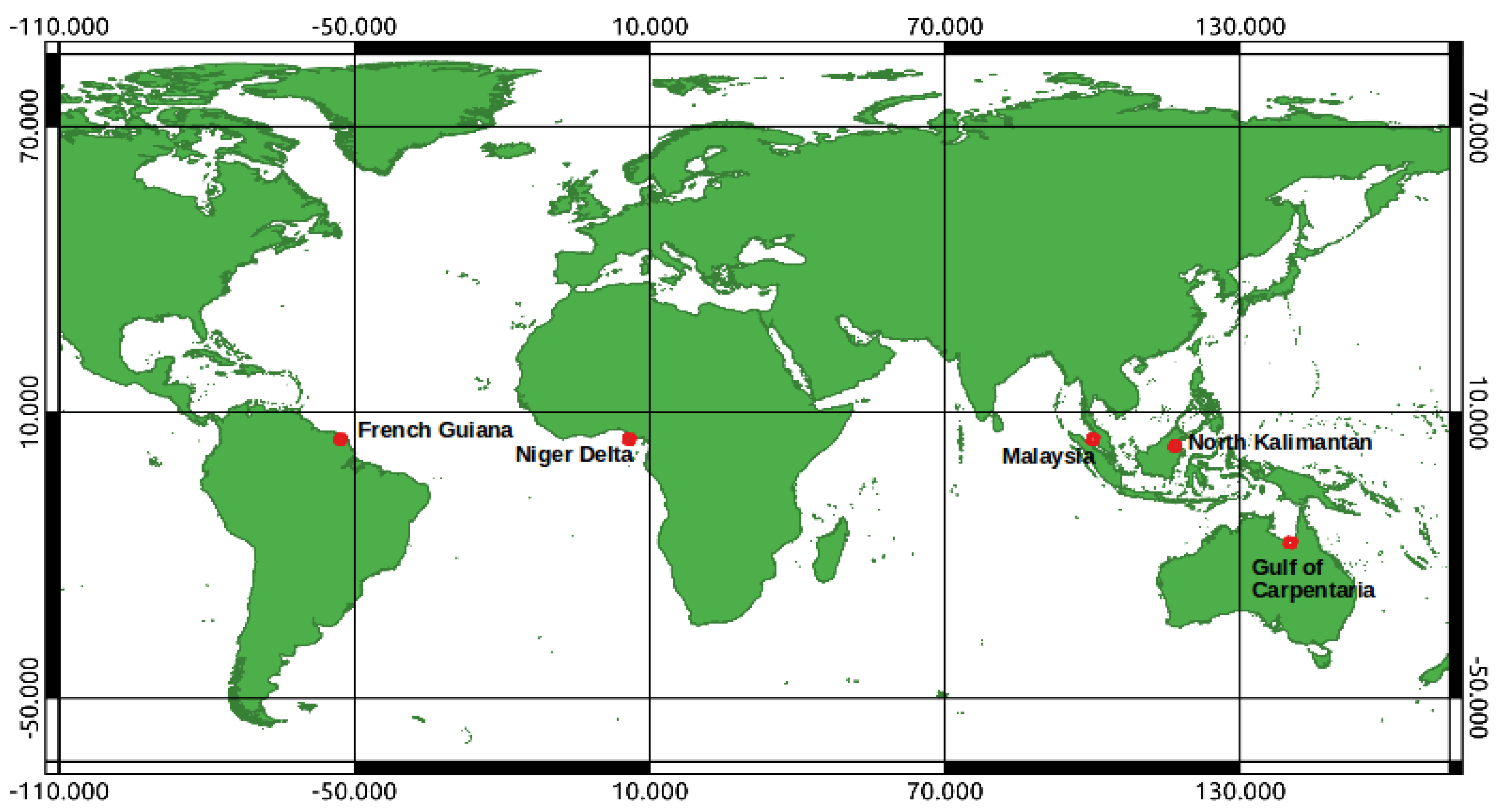
Table 1.
Description of the five study sites.
| Study Site | Path/Row | Rainfall (mm/year) | Species | No. of Scenes |
|---|---|---|---|---|
| Niger Delta | 189/57 | 3000–4500 [14,33] | Rhizophora racemosa, R. mangle, R. harrisonii [34,35] | 163 |
| French Guiana | 227/57 | 2000–3000 [36,37] | Avicennia germinans, Laguncularia racemosa, Rhizophora sp. [36,38] | 203 |
| Borneo | 117/58 | 1800–3000 [39,40] | Avicennia sp., Sonneratia sp. [40,41] | 392 |
| Malaysia | 128/57 | 2000–2800 [42,43] | Rhizophora apiculata, Rhizophora mucronata [44,45] | 605 |
| Australia | 99/72 | 600–1800 [46] | Avicennia marina, Rhizophora stylosa [46,47] | 890 |
Table 2.
Number of training samples used for each site, for each class. A total of 500,000 random samples were taken for each class, before only the stable models for the training year (2010) were screened out and used to train the classifiers.
Table 2.
Number of training samples used for each site, for each class. A total of 500,000 random samples were taken for each class, before only the stable models for the training year (2010) were screened out and used to train the classifiers.
| Study Site | Other Land | Water | Mangroves | Total |
|---|---|---|---|---|
| Niger Delta | 217,348 | 422,090 | 413,954 | 1,053,392 |
| French Guiana | 310,546 | 477,790 | 204,861 | 993,197 |
| Borneo | 315,859 | 497,380 | 269,027 | 1,082,266 |
| Malaysia | 248,994 | 499,396 | 465,032 | 1,213,422 |
| Australia | 91,057 | 457,280 | 227,171 | 775,508 |
| Total | 1,183,804 | 2,353,936 | 1,580,045 | 5,117,785 |
Table 3.
Results of the spatiotemporal accuracy assessment for COLD over the five study sites, for the overall classifier.
Table 3.
Results of the spatiotemporal accuracy assessment for COLD over the five study sites, for the overall classifier.
| Reference | ||||||
|---|---|---|---|---|---|---|
| Mangrove | Water | Other | Total | User’s (%) | ||
| Classifier | Mangrove | 3398 | 153 | 863 | 4414 | 77.0 |
| Water | 156 | 14,727 | 1448 | 16,331 | 90.2 | |
| Other | 128 | 56 | 13,627 | 13,811 | 98.7 | |
| Total | 3682 | 14,936 | 15,938 | 34,556 | ||
| Producer’s (%) | 92.3 | 98.6 | 85.5 | 92.7 |
Table 4.
Results of spatiotemporal accuracy assessment for the Niger Delta.
| Reference | ||||||
|---|---|---|---|---|---|---|
| Mangrove | Water | Other | Total | User’s (%) | ||
| Classifier | Mangrove | 1026 | 29 | 41 | 1096 | 93.6 |
| Water | 3 | 2537 | 2 | 2542 | 99.8 | |
| Other | 24 | 12 | 2131 | 2167 | 98.3 | |
| Total | 1053 | 2578 | 2174 | 5805 | ||
| Producer’s (%) | 97.4 | 98.4 | 98.0 | 98.1 |
Table 5.
Results of spatiotemporal accuracy assessment for French Guiana.
| Reference | ||||||
|---|---|---|---|---|---|---|
| Mangrove | Water | Other | Total | User’s (%) | ||
| Classifier | Mangrove | 504 | 35 | 285 | 824 | 61.2 |
| Water | 16 | 3272 | 20 | 3308 | 98.9 | |
| Other | 34 | 8 | 3330 | 3372 | 98.8 | |
| Total | 554 | 3315 | 3635 | 7504 | ||
| Producer’s (%) | 91.0 | 98.7 | 91.6 | 96.0 |
Table 6.
Results of spatiotemporal accuracy assessment for North Kalimantan, Borneo island.
| Reference | ||||||
|---|---|---|---|---|---|---|
| Mangrove | Water | Other | Total | User’s (%) | ||
| Classifier | Mangrove | 434 | 45 | 390 | 869 | 49.9 |
| Water | 46 | 2892 | 206 | 3144 | 92.0 | |
| Other | 11 | 17 | 2640 | 2668 | 99.0 | |
| Total | 491 | 2954 | 3236 | 6681 | ||
| Producer’s (%) | 88.4 | 97.9 | 81.6 | 92.3 |
Table 7.
Results of spatiotemporal accuracy assessment for the Matang Forest Reserve, Malaysia.
| Reference | ||||||
|---|---|---|---|---|---|---|
| Mangrove | Water | Other | Total | User’s (%) | ||
| Classifier | Mangrove | 1089 | 37 | 65 | 1191 | 91.4 |
| Water | 19 | 3035 | 30 | 3084 | 98.4 | |
| Other | 22 | 6 | 2654 | 2682 | 99.0 | |
| Total | 1130 | 3078 | 2749 | 6957 | ||
| Producer’s (%) | 96.4 | 98.6 | 96.5 | 97.5 |
Table 8.
Results of spatiotemporal accuracy assessment for the Gulf of Carpentaria, Northern Australia.
Table 8.
Results of spatiotemporal accuracy assessment for the Gulf of Carpentaria, Northern Australia.
| Reference | ||||||
|---|---|---|---|---|---|---|
| Mangrove | Water | Other | Total | User’s (%) | ||
| Classifier | Mangrove | 345 | 7 | 82 | 343 | 79.5 |
| Water | 72 | 2991 | 1190 | 4253 | 70.3 | |
| Other | 37 | 13 | 2872 | 2922 | 98.3 | |
| Total | 454 | 3011 | 4144 | 7609 | ||
| Producer’s (%) | 76.0 | 99.3 | 69.3 | 86.1 |
Publisher’s Note: MDPI stays neutral with regard to jurisdictional claims in published maps and institutional affiliations. |
© 2021 by the authors. Licensee MDPI, Basel, Switzerland. This article is an open access article distributed under the terms and conditions of the Creative Commons Attribution (CC BY) license (https://creativecommons.org/licenses/by/4.0/).
Share and Cite
MDPI and ACS Style
Awty-Carroll, K.; Bunting, P.; Hardy, A.; Bell, G. Evaluation of the Continuous Monitoring of Land Disturbance Algorithm for Large-Scale Mangrove Classification. Remote Sens. 2021, 13, 3978. https://doi.org/10.3390/rs13193978
AMA Style
Awty-Carroll K, Bunting P, Hardy A, Bell G. Evaluation of the Continuous Monitoring of Land Disturbance Algorithm for Large-Scale Mangrove Classification. Remote Sensing. 2021; 13(19):3978. https://doi.org/10.3390/rs13193978
Chicago/Turabian StyleAwty-Carroll, Katie, Pete Bunting, Andy Hardy, and Gemma Bell. 2021. "Evaluation of the Continuous Monitoring of Land Disturbance Algorithm for Large-Scale Mangrove Classification" Remote Sensing 13, no. 19: 3978. https://doi.org/10.3390/rs13193978
Note that from the first issue of 2016, this journal uses article numbers instead of page numbers. See further details here.